Fantastic Measures of Generalization — That Actually Work (part 1) #AI

#A.I.

In the next few posts, I am going to discuss how to use the generalization metrics included in the open-source weightwatcher tool. The goal is to develop a general-purpose tool can that you can use, among other things, to predict (tends in) the test accuracy of a Deep Neural Network — without access to the test data — or even training data!

WeightWatcher is a work in progress, based on research into Why Deep Learning Works, and has been featured in venures like ICML, KDD, JMLR and Nature Communications.

Before we start, let me just say that it is very difficult to develop general-purpose metrics that can work for any arbitrary DNN (DNN), and, also, maintains a tool that is also back comparable with all of our work to be 100% reproducible. I hope the tool is useful to you, and we rely upon your feedback (positive and negative ) to improve the tool. so if it works for you, please let me. If not, feel free to post an issue on the Github site. Thanks again for the interest!

Given this, the first metrics we will look at will be the

Random Distance Metrics

How is it even possible to predict the generalization accuracy of a DNN without even needing the test data ? Or at least trends ? The basic idea is simple; for each later weight matrix, measure how non-random it is. After all, the more information the layer learns, the less random it should be.

What are some choices for such a layer capacity metric:

• Matrix Entropy:
• Distance from the initial weight matrix: (and variants of this)
• DIvergence from the ESD of the randomized weight matrix:

Matrix Entropy

We define in terms of the eigenvalues of the layer correlation matrix

.

So the matrix entropy i is both a measure of layer randomness and a measure of correlation.

In our JMLR paper, however, we show that while the Matrix Entropy does decrease during training, it is not particularly informative. Still, I mention it here for completeness. (And in the next post, I will discuss the Stable Rank; stay tuned)

Distance from Init:

The next metric to consider is the Frobenius norm of the difference between the layer weight matrix and it’s specific, initialized, random value . Note, however, that this metric requires that you actually have the initial layer matrices (which we did not for our Nature paper)

The weightwatcher tool supports this metric with the distance method:

import weightwatcher as ww
watcher = ww.watcher(model=your_model)
distance_from_init = watcher.distances(your_model, init_model)

where init_model is your model, with the original, actual, initial weight matrices.

In our most recent paper, we evaluated the distance_from_init method as a generalization metric in great detal, however, in order to cut the paper down to submit (which I really hate doing), we had to remove most of this discussion, and only a table in the appendix remained. I may redo this paper, and revert it to the long form, at some point. For now, I will just present some results from that study here, that are unpublished.

These are the raw results for the task1 and task2 sets of models, described in the paper. Breifly we were given about 100 pretrained models, group into 2 tasks (corresponding to 2 different architectures), and then subgrouped again (by the number of layers in each set). Here, we see how the distance_from_init metric correlates against the given test accuracies–and it’s pretty good most of the time. But’s not the best metric in general.

The problem with this simple approach is it is not going to be useful if your models are overfit because the distance from init increases over time anyway–and this is exactly what we think is happening in the task1 models from this NeurIPS contest. But it is a good sanity check on your models during training, and can be used with other metrics as a diagnostic indicator.

The are a few variants of this distance metric, depending on how one defines the distance. These include:

1. Frobenius norm distance.
2. Cosine distance
3. CKA distance

Currently, weightwatcher 0.5.5 only supports (1), but in the next minor release, we plan to include both (2) & (3).

Distance from Random: (rand_distance)

With the new rand_distance metric, we mean something very different from the distance_from_init. Above, we used the original instantiation of the $latex \mathbf{W}_{init}
&bg=ffffff$, and constructed an element-wise distance metric. The rand_distance metric, in contrast:

• Does not require the original, initial weight matrics
• Is not an element-wise metric, but, instead, is a distributional metric

So this metric is defined in terms of a distance between the distributions of the eigenvalues (i..e the ESDs) of the layer matrix and its random counterpart
.

rand_distance = jensen_shannon_distance(esd, rand_esd)

For weightwatcher, we choose to use the Jensen-Shannon divergence for this:

def jensen_shannon_distance(p, q):
    m = (p + q) / 2
    divergence = (sp.stats.entropy(p, m) + sp.stats.entropy(q, m)) / 2
    distance = np.sqrt(divergence)
    return distance

Moreover, there are 2 ways to construct the random layer matrix $\mathbf{W}_{rand}&bg=ffffff$ metric:

1. Take any (Gaussian) Random Matrix, with the same aspect ratio as the layer weight matrix
2. Permute (shuffle) the elements of

While at first glance, these may seem the same, in fact, in practice, they can be quite different. This is because while every (Normal) Random Matrix has the same ESD (up to finite size effects), the Marchenko-Pastur (MP) distribution, if the actual contains any usually large elements , then it’s ESD will behave like a Heavy-Tailed Random Matrix, and look very different from it’s random MP counterpart. For more details, see our JMLR paper.

Indeed, when contains usually large elements, we call these Correlation Traps. Now, I have conjectured, in an earlier post, that such Correlation Traps may be a indication of a layer being overtrained. However, some research suggests the opposite, and, that, in-fact, such large elements are needed for large, modern NLP models. The jury is still out on this, however, the weightwatcher tool can be used to resolve this question since it can easily identify such Correlation Traps in every layer. I look forward to seeing the final conclusion.

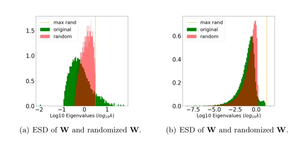
The take-a-way here is that, when a layer is well trained, we expect the ESD of the layer to be significantly different from the ESD its randomized, shuffled form. Let’s compare 2 cases:

In case (a), the original ESD (green) looks significantly different from its randomized ESD (red).
In case (b), however, the original the randomized ESDs are much more similar. So we expect case (a) to be more well trained than case (b).

To compute the rand_distance metric, simply specify the randomize=True option, and it will be available as a layer metric in the details dataframe

import weightwatcher as ww
watcher = ww.watcher(model=your_model)
details = watcher.analyze(randomize=True)
avg_rand_distance = details.rand_distance.mean()

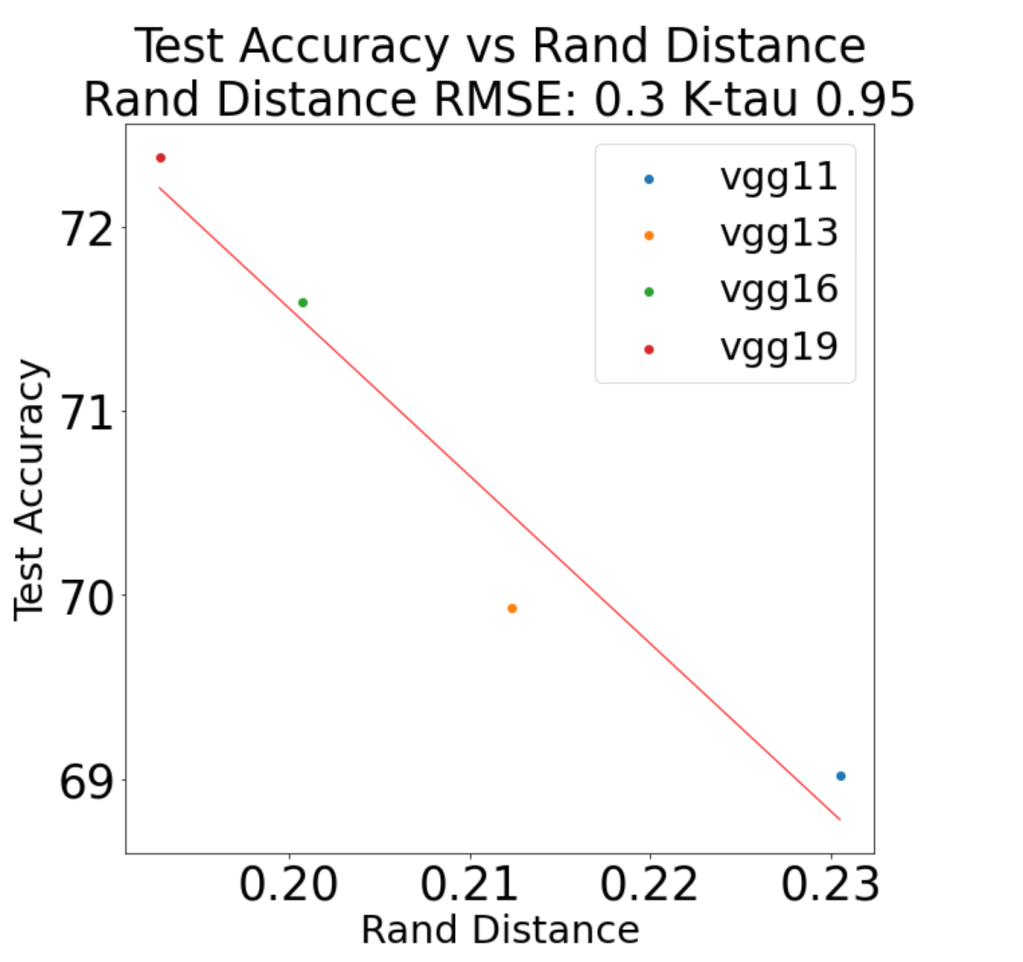
Finally, let’s see how well the rand_distance metric actually works to predict trends in the test accuracy for a well known set of pretrained models, the VGG series. Similar to the analysis in our Nature paper, we consider how well the average rand_distance metric is correlated with the reported top1 errors of the series of VGG models: VGG11, VGG13, VGG16, and VGG19

Actually this is pretty good, and comparable to the results for the weightwatcher powerlaw metric weighted-alpha ().  But for reasons I don’t yet understand, however, it does not work so well for the VGG_BN models (VGG with BatchNormalization).  Never-the-less, I am hoping it may be useful to you, and I would love to hear if it is working for you or not.  To help get started, the above results can be reproduced using weightwatcher 0.5.5 using the WWVGG-TestRandDistance.ipynb Jupyter Notebook in the WeightWatcher GitHub repo.

I’ll end part 1 of this series of blog posts with a comparison between the new rand_distance metric and the weighwatcher alpha metric, for all the layers VGG19.

(Note, I am not using the ww2x option for this analysis, but if you want to reproduce the Nature results, use ww2x=True. If you don’t , you may get crazy-large alphas that are incorrect–I will show in the next post I will discuss the alpha powerlaw (PL) estimates in more detail.)

When the weightwatcher alpha < 5, this means that the layers are Heavy Tailed and therefore well trained, and, as expected, alpha is correlated with the rand_distance metric. As expected!

I hope this has been useful to you and that you will try out the weightwather tool

pip install weightwatcher 

Give it a try. And please give me feedback if it is useful. And, if interested in getting involved or just learning more, ping me to join our Slack channel. And if you need help with AI, reach out. #talkToChuck #theAIguy

via https://AIupNow.com

Charles H Martin, PhD, Khareem Sudlow