Regression is a modeling task that involves predicting a numerical value given an input.
Algorithms used for regression tasks are also referred to as “regression” algorithms, with the most widely known and perhaps most successful being linear regression.
Linear regression fits a line or hyperplane that best describes the linear relationship between inputs and the target numeric value. If the data contains outlier values, the line can become biased, resulting in worse predictive performance. Robust regression refers to a suite of algorithms that are robust in the presence of outliers in training data.
In this tutorial, you will discover robust regression algorithms for machine learning.
After completing this tutorial, you will know:
- Robust regression algorithms can be used for data with outliers in the input or target values.
- How to evaluate robust regression algorithms for a regression predictive modeling task.
- How to compare robust regression algorithms using their line of best fit on the dataset.
Let’s get started.

Robust Regression for Machine Learning in Python
Photo by Lenny K Photography, some rights reserved.
Tutorial Overview
This tutorial is divided into four parts; they are:
- Regression With Outliers
- Regression Dataset With Outliers
- Robust Regression Algorithms
- Compare Robust Regression Algorithms
Regression With Outliers
Regression predictive modeling involves predicting a numeric variable given some input, often numerical input.
Machine learning algorithms used for regression predictive modeling tasks are also referred to as “regression” or “regression algorithms.” The most common method is linear regression.
Many regression algorithms are linear in that they assume that the relationship between the input variable or variables and the target variable is linear, such as a line in two-dimensions, a plane in three dimensions, and a hyperplane in higher dimensions. This is a reasonable assumption for many prediction tasks.
Linear regression assumes that the probability distribution of each variable is well behaved, such as has a Gaussian distribution. The less well behaved the probability distribution for a feature is in a dataset, the less likely that linear regression will find a good fit.
A specific problem with the probability distribution of variables when using linear regression is outliers. These are observations that are far outside the expected distribution. For example, if a variable has a Gaussian distribution, then an observation that is 3 or 4 (or more) standard deviations from the mean is considered an outlier.
A dataset may have outliers on either the input variables or the target variable, and both can cause problems for a linear regression algorithm.
Outliers in a dataset can skew summary statistics calculated for the variable, such as the mean and standard deviation, which in turn can skew the model towards the outlier values, away from the central mass of observations. This results in models that try to balance performing well on outliers and normal data, and performing worse on both overall.
The solution instead is to use modified versions of linear regression that specifically address the expectation of outliers in the dataset. These methods are referred to as robust regression algorithms.
Regression Dataset With Outliers
We can define a synthetic regression dataset using the make_regression() function.
In this case, we want a dataset that we can plot and understand easily. This can be achieved by using a single input variable and a single output variable. We don’t want the task to be too easy, so we will add a large amount of statistical noise.
...
X, y = make_regression(n_samples=100, n_features=1, tail_strength=0.9, effective_rank=1, n_informative=1, noise=3, bias=50, random_state=1)
Once we have the dataset, we can augment it by adding outliers. Specifically, we will add outliers to the input variables.
This can be done by changing some of the input variables to have a value that is a factor of the number of standard deviations away from the mean, such as 2-to-4. We will add 10 outliers to the dataset.
# add some artificial outliers
seed(1)
for i in range(10):
        factor = randint(2, 4)
        if random() > 0.5:
                X[i] += factor * X.std()
        else:
                X[i] -= factor * X.std()
We can tie this together into a function that will prepare the dataset. This function can then be called and we can plot the dataset with the input values on the x-axis and the target or outcome on the y-axis.
The complete example of preparing and plotting the dataset is listed below.
# create a regression dataset with outliers
from random import random
from random import randint
from random import seed
from sklearn.datasets import make_regression
from matplotlib import pyplot

# prepare the dataset
def get_dataset():
        X, y = make_regression(n_samples=100, n_features=1, tail_strength=0.9, effective_rank=1, n_informative=1, noise=3, bias=50, random_state=1)
        # add some artificial outliers
        seed(1)
        for i in range(10):
                factor = randint(2, 4)
                if random() > 0.5:
                        X[i] += factor * X.std()
                else:
                        X[i] -= factor * X.std()
        return X, y

# load dataset
X, y = get_dataset()
# summarize shape
print(X.shape, y.shape)
# scatter plot of input vs output
pyplot.scatter(X, y)
pyplot.show()
Running the example creates the synthetic regression dataset and adds outlier values.
The dataset is then plotted, and we can clearly see the linear relationship in the data, with statistical noise, and a modest number of outliers as points far from the main mass of data.
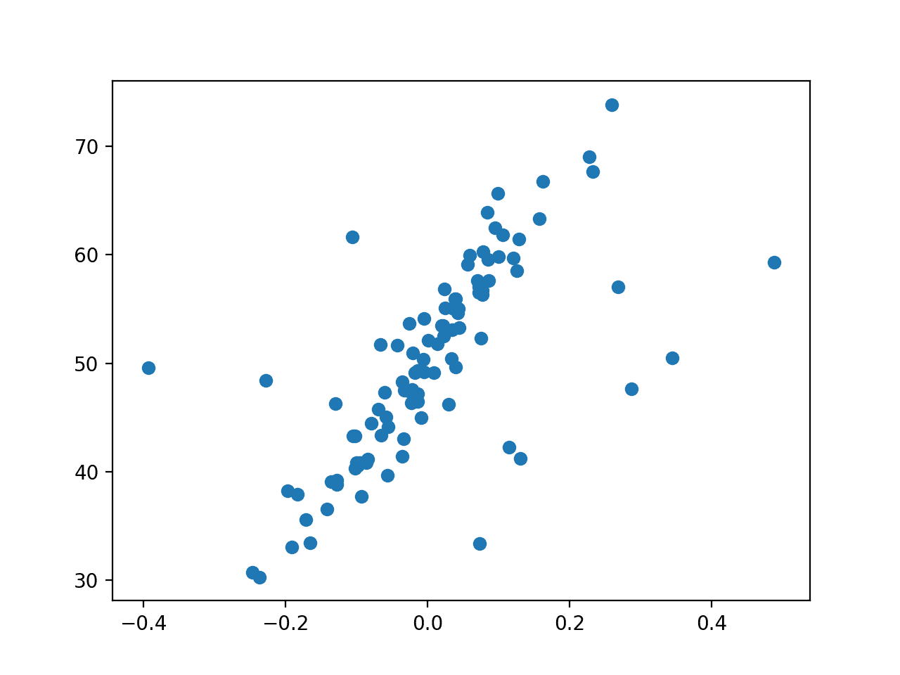
Scatter Plot of Regression Dataset With Outliers
Now that we have a dataset, let’s fit different regression models on it.
Robust Regression Algorithms
In this section, we will consider different robust regression algorithms for the dataset.
Linear Regression (not robust)
Before diving into robust regression algorithms, let’s start with linear regression.
We can evaluate linear regression using repeated k-fold cross-validation on the regression dataset with outliers. We will measure mean absolute error and this will provide a lower bound on model performance on this task that we might expect some robust regression algorithms to out-perform.
# evaluate a model
def evaluate_model(X, y, model):
        # define model evaluation method
        cv = RepeatedKFold(n_splits=10, n_repeats=3, random_state=1)
        # evaluate model
        scores = cross_val_score(model, X, y, scoring='neg_mean_absolute_error', cv=cv, n_jobs=-1)
        # force scores to be positive
        return absolute(scores)
We can also plot the model’s line of best fit on the dataset. To do this, we first fit the model on the entire training dataset, then create an input dataset that is a grid across the entire input domain, make a prediction for each, then draw a line for the inputs and predicted outputs.
This plot shows how the model “sees” the problem, specifically the relationship between the input and output variables. The idea is that the line will be skewed by the outliers when using linear regression.
# plot the dataset and the model's line of best fit
def plot_best_fit(X, y, model):
        # fut the model on all data
        model.fit(X, y)
        # plot the dataset
        pyplot.scatter(X, y)
        # plot the line of best fit
        xaxis = arange(X.min(), X.max(), 0.01)
        yaxis = model.predict(xaxis.reshape((len(xaxis), 1)))
        pyplot.plot(xaxis, yaxis, color='r')
        # show the plot
        pyplot.title(type(model).__name__)
        pyplot.show()
Tying this together, the complete example for linear regression is listed below.
# linear regression on a dataset with outliers
from random import random
from random import randint
from random import seed
from numpy import arange
from numpy import mean
from numpy import std
from numpy import absolute
from sklearn.datasets import make_regression
from sklearn.linear_model import LinearRegression
from sklearn.model_selection import cross_val_score
from sklearn.model_selection import RepeatedKFold
from matplotlib import pyplot

# prepare the dataset
def get_dataset():
        X, y = make_regression(n_samples=100, n_features=1, tail_strength=0.9, effective_rank=1, n_informative=1, noise=3, bias=50, random_state=1)
        # add some artificial outliers
        seed(1)
        for i in range(10):
                factor = randint(2, 4)
                if random() > 0.5:
                        X[i] += factor * X.std()
                else:
                        X[i] -= factor * X.std()
        return X, y

# evaluate a model
def evaluate_model(X, y, model):
        # define model evaluation method
        cv = RepeatedKFold(n_splits=10, n_repeats=3, random_state=1)
        # evaluate model
        scores = cross_val_score(model, X, y, scoring='neg_mean_absolute_error', cv=cv, n_jobs=-1)
        # force scores to be positive
        return absolute(scores)

# plot the dataset and the model's line of best fit
def plot_best_fit(X, y, model):
        # fut the model on all data
        model.fit(X, y)
        # plot the dataset
        pyplot.scatter(X, y)
        # plot the line of best fit
        xaxis = arange(X.min(), X.max(), 0.01)
        yaxis = model.predict(xaxis.reshape((len(xaxis), 1)))
        pyplot.plot(xaxis, yaxis, color='r')
        # show the plot
        pyplot.title(type(model).__name__)
        pyplot.show()

# load dataset
X, y = get_dataset()
# define the model
model = LinearRegression()
# evaluate model
results = evaluate_model(X, y, model)
print('Mean MAE: %.3f (%.3f)' % (mean(results), std(results)))
# plot the line of best fit
plot_best_fit(X, y, model)
Running the example first reports the mean MAE for the model on the dataset.
We can see that linear regression achieves a MAE of about 5.2 on this dataset, providing an upper-bound in error.
Mean MAE: 5.260 (1.149)
Next, the dataset is plotted as a scatter plot showing the outliers and this is overlaid with the line of best fit from the linear regression algorithm.
In this case, we can see that the line of best fit is not aligning with the data and it has been skewed by the outliers. In turn, we expect this has caused the model to have a worse-than-expected performance on the dataset.
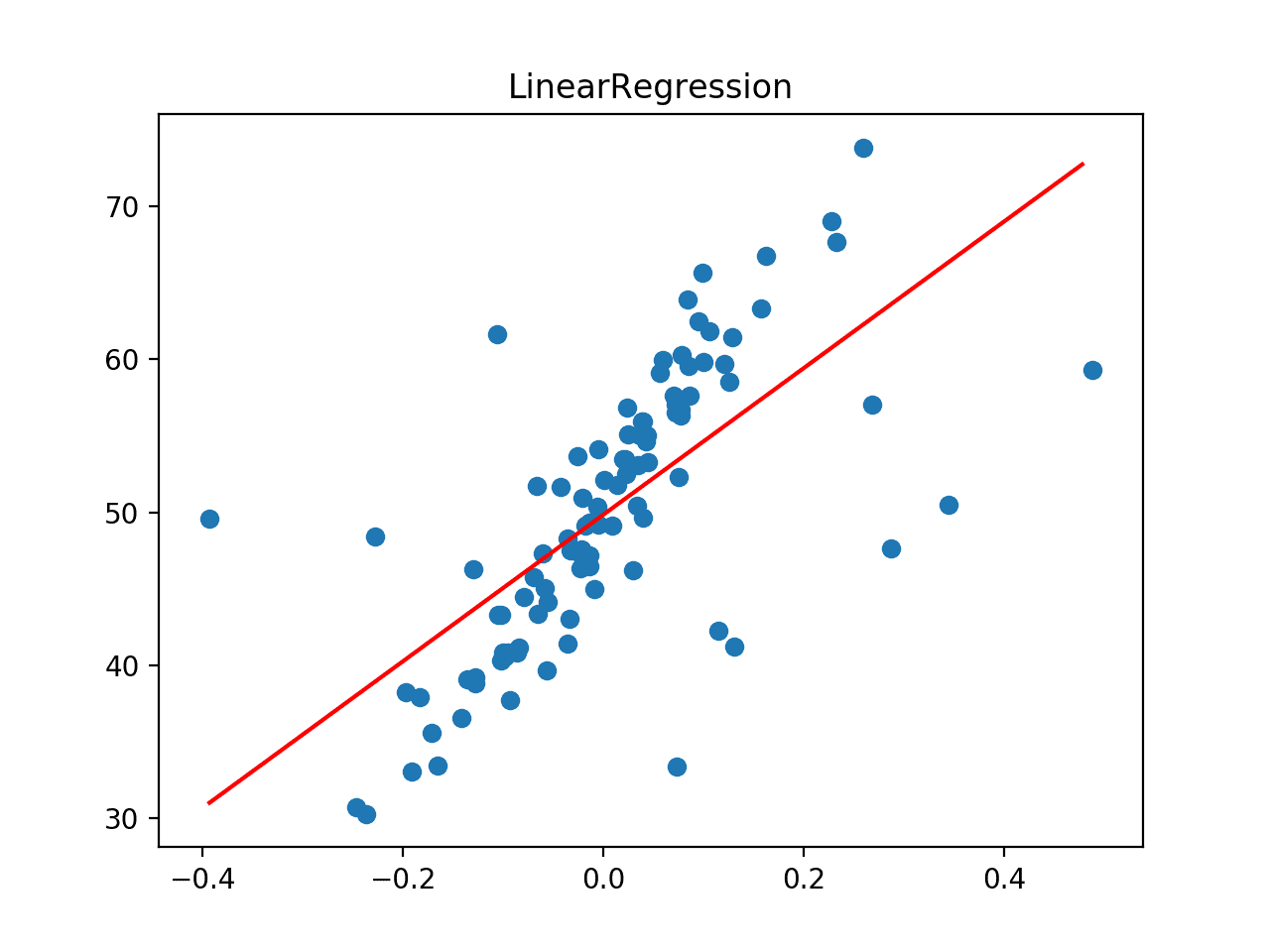
Line of Best Fit for Linear Regression on a Dataset with Outliers
Huber Regression
Huber regression is a type of robust regression that is aware of the possibility of outliers in a dataset and assigns them less weight than other examples in the dataset.
We can use Huber regression via the HuberRegressor class in scikit-learn. The “epsilon” argument controls what is considered an outlier, where smaller values consider more of the data outliers, and in turn, make the model more robust to outliers. The default is 1.35.
The example below evaluates Huber regression on the regression dataset with outliers, first evaluating the model with repeated cross-validation and then plotting the line of best fit.
# huber regression on a dataset with outliers
from random import random
from random import randint
from random import seed
from numpy import arange
from numpy import mean
from numpy import std
from numpy import absolute
from sklearn.datasets import make_regression
from sklearn.linear_model import HuberRegressor
from sklearn.model_selection import cross_val_score
from sklearn.model_selection import RepeatedKFold
from matplotlib import pyplot

# prepare the dataset
def get_dataset():
        X, y = make_regression(n_samples=100, n_features=1, tail_strength=0.9, effective_rank=1, n_informative=1, noise=3, bias=50, random_state=1)
        # add some artificial outliers
        seed(1)
        for i in range(10):
                factor = randint(2, 4)
                if random() > 0.5:
                        X[i] += factor * X.std()
                else:
                        X[i] -= factor * X.std()
        return X, y

# evaluate a model
def evaluate_model(X, y, model):
        # define model evaluation method
        cv = RepeatedKFold(n_splits=10, n_repeats=3, random_state=1)
        # evaluate model
        scores = cross_val_score(model, X, y, scoring='neg_mean_absolute_error', cv=cv, n_jobs=-1)
        # force scores to be positive
        return absolute(scores)

# plot the dataset and the model's line of best fit
def plot_best_fit(X, y, model):
        # fut the model on all data
        model.fit(X, y)
        # plot the dataset
        pyplot.scatter(X, y)
        # plot the line of best fit
        xaxis = arange(X.min(), X.max(), 0.01)
        yaxis = model.predict(xaxis.reshape((len(xaxis), 1)))
        pyplot.plot(xaxis, yaxis, color='r')
        # show the plot
        pyplot.title(type(model).__name__)
        pyplot.show()

# load dataset
X, y = get_dataset()
# define the model
model = HuberRegressor()
# evaluate model
results = evaluate_model(X, y, model)
print('Mean MAE: %.3f (%.3f)' % (mean(results), std(results)))
# plot the line of best fit
plot_best_fit(X, y, model)
Running the example first reports the mean MAE for the model on the dataset.
We can see that Huber regression achieves a MAE of about 4.435 on this dataset, outperforming the linear regression model in the previous section.
Mean MAE: 4.435 (1.868)
Next, the dataset is plotted as a scatter plot showing the outliers and this is overlaid with the line of best fit from the algorithm.
In this case, we can see that the line of best fit is better aligned with the main body of the data, and does not appear to be obviously influenced by the outliers that are present.
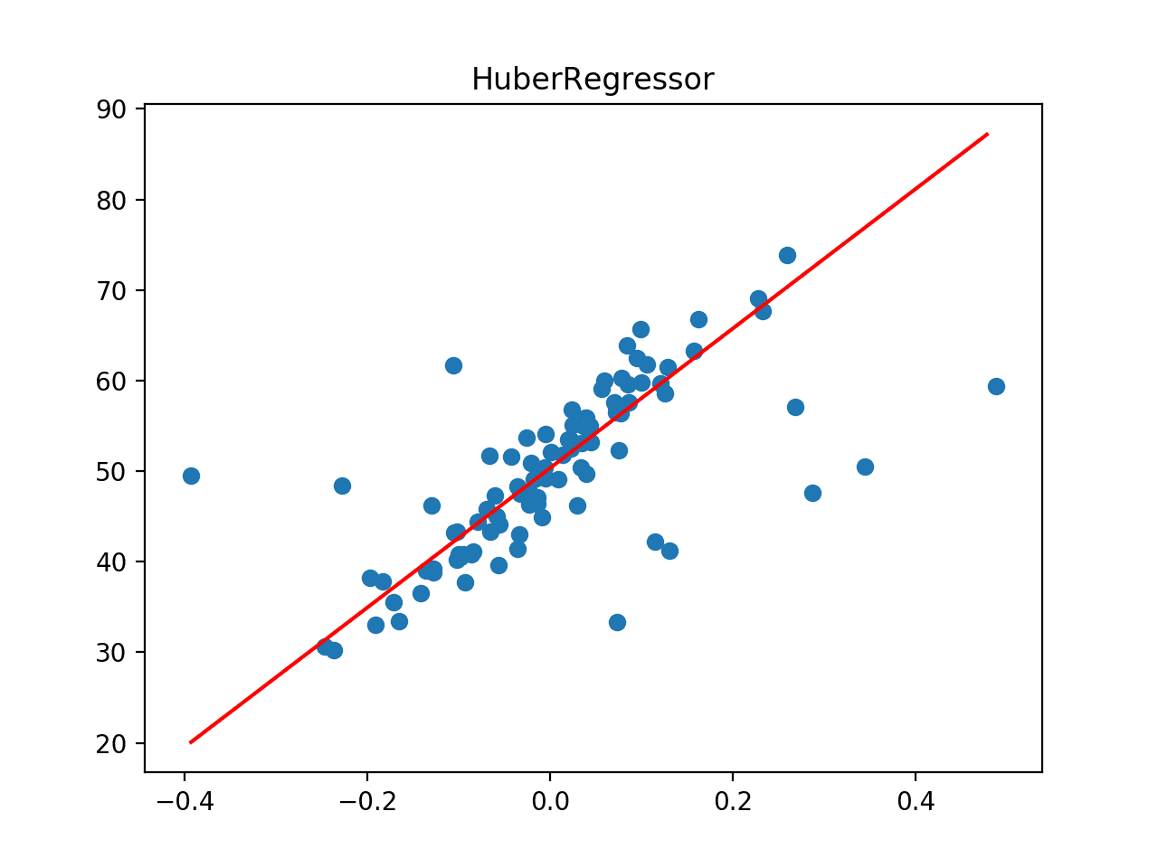
Line of Best Fit for Huber Regression on a Dataset with Outliers
RANSAC Regression
Random Sample Consensus, or RANSAC for short, is another robust regression algorithm.
RANSAC tries to separate data into outliers and inliers and fits the model on the inliers.
The scikit-learn library provides an implementation via the RANSACRegressor class.
The example below evaluates RANSAC regression on the regression dataset with outliers, first evaluating the model with repeated cross-validation and then plotting the line of best fit.
# ransac regression on a dataset with outliers
from random import random
from random import randint
from random import seed
from numpy import arange
from numpy import mean
from numpy import std
from numpy import absolute
from sklearn.datasets import make_regression
from sklearn.linear_model import RANSACRegressor
from sklearn.model_selection import cross_val_score
from sklearn.model_selection import RepeatedKFold
from matplotlib import pyplot

# prepare the dataset
def get_dataset():
        X, y = make_regression(n_samples=100, n_features=1, tail_strength=0.9, effective_rank=1, n_informative=1, noise=3, bias=50, random_state=1)
        # add some artificial outliers
        seed(1)
        for i in range(10):
                factor = randint(2, 4)
                if random() > 0.5:
                        X[i] += factor * X.std()
                else:
                        X[i] -= factor * X.std()
        return X, y

# evaluate a model
def evaluate_model(X, y, model):
        # define model evaluation method
        cv = RepeatedKFold(n_splits=10, n_repeats=3, random_state=1)
        # evaluate model
        scores = cross_val_score(model, X, y, scoring='neg_mean_absolute_error', cv=cv, n_jobs=-1)
        # force scores to be positive
        return absolute(scores)

# plot the dataset and the model's line of best fit
def plot_best_fit(X, y, model):
        # fut the model on all data
        model.fit(X, y)
        # plot the dataset
        pyplot.scatter(X, y)
        # plot the line of best fit
        xaxis = arange(X.min(), X.max(), 0.01)
        yaxis = model.predict(xaxis.reshape((len(xaxis), 1)))
        pyplot.plot(xaxis, yaxis, color='r')
        # show the plot
        pyplot.title(type(model).__name__)
        pyplot.show()

# load dataset
X, y = get_dataset()
# define the model
model = RANSACRegressor()
# evaluate model
results = evaluate_model(X, y, model)
print('Mean MAE: %.3f (%.3f)' % (mean(results), std(results)))
# plot the line of best fit
plot_best_fit(X, y, model)
Running the example first reports the mean MAE for the model on the dataset.
We can see that RANSAC regression achieves a MAE of about 4.454 on this dataset, outperforming the linear regression model but perhaps not Huber regression.
Mean MAE: 4.454 (2.165)
Next, the dataset is plotted as a scatter plot showing the outliers, and this is overlaid with the line of best fit from the algorithm.
In this case, we can see that the line of best fit is aligned with the main body of the data, perhaps even better than the plot for Huber regression.
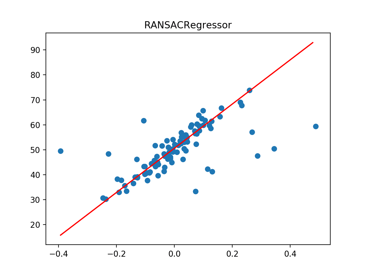
Line of Best Fit for RANSAC Regression on a Dataset with Outliers
Theil Sen Regression
Theil Sen regression involves fitting multiple regression models on subsets of the training data and combining the coefficients together in the end.
The scikit-learn provides an implementation via the TheilSenRegressor class.
The example below evaluates Theil Sen regression on the regression dataset with outliers, first evaluating the model with repeated cross-validation and then plotting the line of best fit.
# theilsen regression on a dataset with outliers
from random import random
from random import randint
from random import seed
from numpy import arange
from numpy import mean
from numpy import std
from numpy import absolute
from sklearn.datasets import make_regression
from sklearn.linear_model import TheilSenRegressor
from sklearn.model_selection import cross_val_score
from sklearn.model_selection import RepeatedKFold
from matplotlib import pyplot

# prepare the dataset
def get_dataset():
        X, y = make_regression(n_samples=100, n_features=1, tail_strength=0.9, effective_rank=1, n_informative=1, noise=3, bias=50, random_state=1)
        # add some artificial outliers
        seed(1)
        for i in range(10):
                factor = randint(2, 4)
                if random() > 0.5:
                        X[i] += factor * X.std()
                else:
                        X[i] -= factor * X.std()
        return X, y

# evaluate a model
def evaluate_model(X, y, model):
        # define model evaluation method
        cv = RepeatedKFold(n_splits=10, n_repeats=3, random_state=1)
        # evaluate model
        scores = cross_val_score(model, X, y, scoring='neg_mean_absolute_error', cv=cv, n_jobs=-1)
        # force scores to be positive
        return absolute(scores)

# plot the dataset and the model's line of best fit
def plot_best_fit(X, y, model):
        # fut the model on all data
        model.fit(X, y)
        # plot the dataset
        pyplot.scatter(X, y)
        # plot the line of best fit
        xaxis = arange(X.min(), X.max(), 0.01)
        yaxis = model.predict(xaxis.reshape((len(xaxis), 1)))
        pyplot.plot(xaxis, yaxis, color='r')
        # show the plot
        pyplot.title(type(model).__name__)
        pyplot.show()

# load dataset
X, y = get_dataset()
# define the model
model = TheilSenRegressor()
# evaluate model
results = evaluate_model(X, y, model)
print('Mean MAE: %.3f (%.3f)' % (mean(results), std(results)))
# plot the line of best fit
plot_best_fit(X, y, model)
Running the example first reports the mean MAE for the model on the dataset.
We can see that Theil Sen regression achieves a MAE of about 4.371 on this dataset, outperforming the linear regression model as well as RANSAC and Huber regression.
Mean MAE: 4.371 (1.961)
Next, the dataset is plotted as a scatter plot showing the outliers, and this is overlaid with the line of best fit from the algorithm.
In this case, we can see that the line of best fit is aligned with the main body of the data.
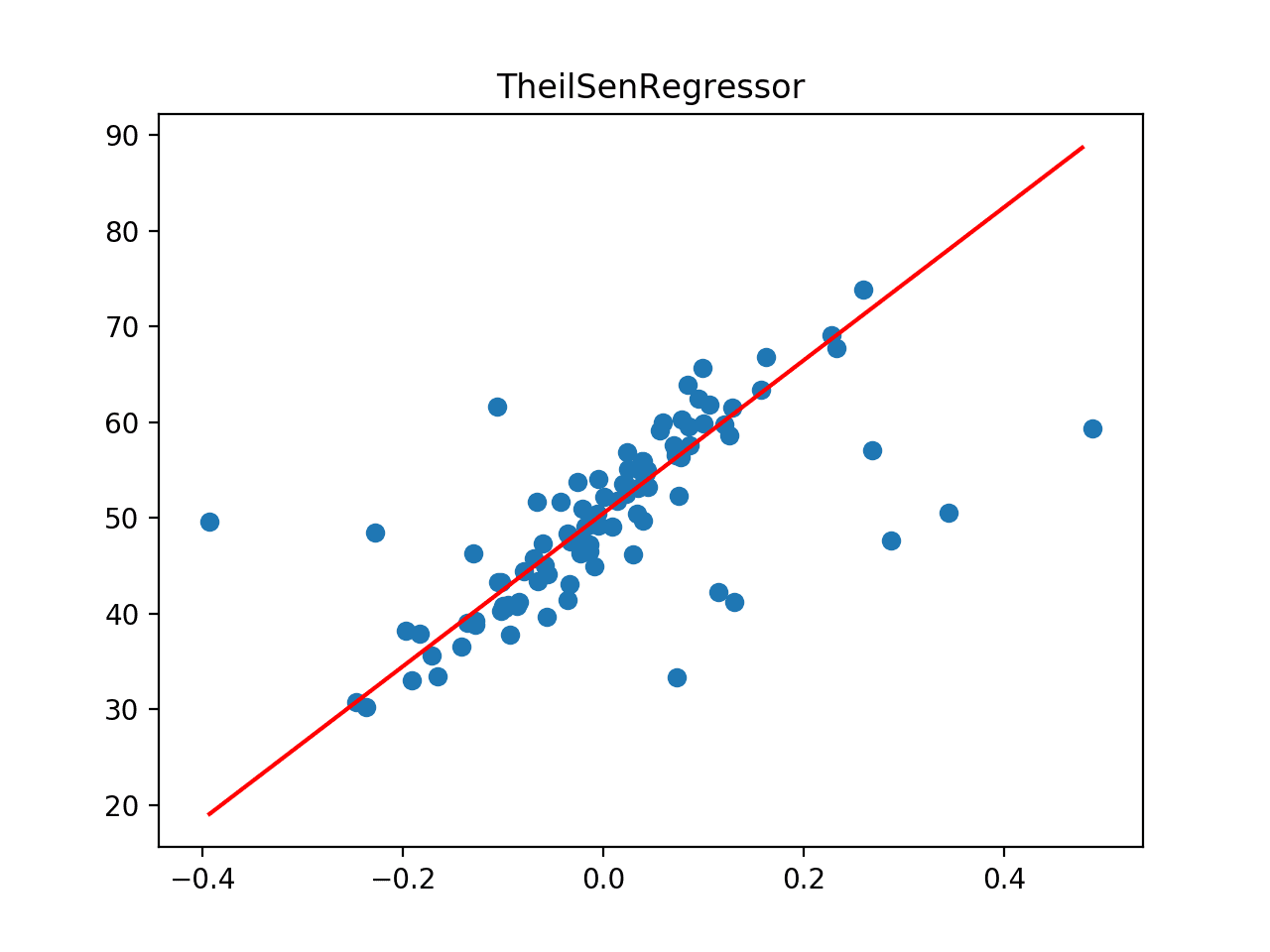
Line of Best Fit for Theil Sen Regression on a Dataset with Outliers
Compare Robust Regression Algorithms
Now that we are familiar with some popular robust regression algorithms and how to use them, we can look at how we might compare them directly.
It can be useful to run an experiment to directly compare the robust regression algorithms on the same dataset. We can compare the mean performance of each method, and more usefully, use tools like a box and whisker plot to compare the distribution of scores across the repeated cross-validation folds.
The complete example is listed below.
# compare robust regression algorithms on a regression dataset with outliers
from random import random
from random import randint
from random import seed
from numpy import mean
from numpy import std
from numpy import absolute
from sklearn.datasets import make_regression
from sklearn.model_selection import cross_val_score
from sklearn.model_selection import RepeatedKFold
from sklearn.linear_model import LinearRegression
from sklearn.linear_model import HuberRegressor
from sklearn.linear_model import RANSACRegressor
from sklearn.linear_model import TheilSenRegressor
from matplotlib import pyplot

# prepare the dataset
def get_dataset():
        X, y = make_regression(n_samples=100, n_features=1, tail_strength=0.9, effective_rank=1, n_informative=1, noise=3, bias=50, random_state=1)
        # add some artificial outliers
        seed(1)
        for i in range(10):
                factor = randint(2, 4)
                if random() > 0.5:
                        X[i] += factor * X.std()
                else:
                        X[i] -= factor * X.std()
        return X, y

# dictionary of model names and model objects
def get_models():
        models = dict()
        models['Linear'] = LinearRegression()
        models['Huber'] = HuberRegressor()
        models['RANSAC'] = RANSACRegressor()
        models['TheilSen'] = TheilSenRegressor()
        return models

# evaluate a model
def evalute_model(X, y, model, name):
        # define model evaluation method
        cv = RepeatedKFold(n_splits=10, n_repeats=3, random_state=1)
        # evaluate model
        scores = cross_val_score(model, X, y, scoring='neg_mean_absolute_error', cv=cv, n_jobs=-1)
        # force scores to be positive
        scores = absolute(scores)
        return scores

# load the dataset
X, y = get_dataset()
# retrieve models
models = get_models()
results = dict()
for name, model in models.items():
        # evaluate the model
        results[name] = evalute_model(X, y, model, name)
        # summarize progress
        print('>%s %.3f (%.3f)' % (name, mean(results[name]), std(results[name])))
# plot model performance for comparison
pyplot.boxplot(results.values(), labels=results.keys(), showmeans=True)
pyplot.show()
Running the example evaluates each model in turn, reporting the mean and standard deviation MAE scores of reach.
Note: your specific results will differ given the stochastic nature of the learning algorithms and evaluation procedure. Try running the example a few times.
We can see some minor differences between these scores and those reported in the previous section, although the differences may or may not be statistically significant. The general pattern of the robust regression methods performing better than linear regression holds, TheilSen achieving better performance than the other methods.
>Linear 5.260 (1.149)
>Huber 4.435 (1.868)
>RANSAC 4.405 (2.206)
>TheilSen 4.371 (1.961)
A plot is created showing a box and whisker plot summarizing the distribution of results for each evaluated algorithm.
We can clearly see the distributions for the robust regression algorithms sitting and extending lower than the linear regression algorithm.
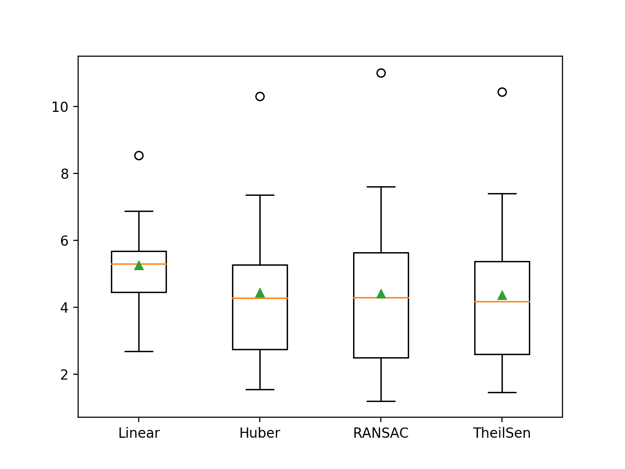
Box and Whisker Plot of MAE Scores for Robust Regression Algorithms
It may also be interesting to compare robust regression algorithms based on a plot of their line of best fit.
The example below fits each robust regression algorithm and plots their line of best fit on the same plot in the context of a scatter plot of the entire training dataset.
# plot line of best for multiple robust regression algorithms
from random import random
from random import randint
from random import seed
from numpy import arange
from sklearn.datasets import make_regression
from sklearn.linear_model import LinearRegression
from sklearn.linear_model import HuberRegressor
from sklearn.linear_model import RANSACRegressor
from sklearn.linear_model import TheilSenRegressor
from matplotlib import pyplot

# prepare the dataset
def get_dataset():
        X, y = make_regression(n_samples=100, n_features=1, tail_strength=0.9, effective_rank=1, n_informative=1, noise=3, bias=50, random_state=1)
        # add some artificial outliers
        seed(1)
        for i in range(10):
                factor = randint(2, 4)
                if random() > 0.5:
                        X[i] += factor * X.std()
                else:
                        X[i] -= factor * X.std()
        return X, y

# dictionary of model names and model objects
def get_models():
        models = list()
        models.append(LinearRegression())
        models.append(HuberRegressor())
        models.append(RANSACRegressor())
        models.append(TheilSenRegressor())
        return models

# plot the dataset and the model's line of best fit
def plot_best_fit(X, y, xaxis, model):
        # fit the model on all data
        model.fit(X, y)
        # calculate outputs for grid across the domain
        yaxis = model.predict(xaxis.reshape((len(xaxis), 1)))
        # plot the line of best fit
        pyplot.plot(xaxis, yaxis, label=type(model).__name__)

# load the dataset
X, y = get_dataset()
# define a uniform grid across the input domain
xaxis = arange(X.min(), X.max(), 0.01)
for model in get_models():
        # plot the line of best fit
        plot_best_fit(X, y, xaxis, model)
# plot the dataset
pyplot.scatter(X, y)
# show the plot
pyplot.title('Robust Regression')
pyplot.legend()
pyplot.show()
Running the example creates a plot showing the dataset as a scatter plot and the line of best fit for each algorithm.
We can clearly see the off-axis line for the linear regression algorithm and the much better lines for the robust regression algorithms that follow the main body of the data.
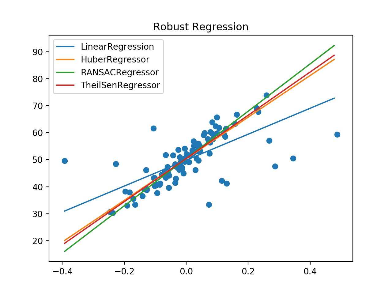
Comparison of Robust Regression Algorithms Line of Best Fit
Further Reading
This section provides more resources on the topic if you are looking to go deeper.
APIs
- Linear Models, scikit-learn.
- sklearn.datasets.make_regression API.
- sklearn.linear_model.LinearRegression API.
- sklearn.linear_model.HuberRegressor API.
- sklearn.linear_model.RANSACRegressor API.
- sklearn.linear_model.TheilSenRegressor API.
Articles
- Robust regression, Wikipedia.
- M-estimator, Wikipedia.
- Random sample consensus, Wikipedia.
- Theil–Sen estimator, Wikipedia.
Summary
In this tutorial, you discovered robust regression algorithms for machine learning.
Specifically, you learned:
- Robust regression algorithms can be used for data with outliers in the input or target values.
- How to evaluate robust regression algorithms for a regression predictive modeling task.
- How to compare robust regression algorithms using their line of best fit on the dataset.
Do you have any questions?
Ask your questions in the comments below and I will do my best to answer.
The post Robust Regression for Machine Learning in Python appeared first on Machine Learning Mastery.
via https://AIupNow.com
Jason Brownlee, Khareem Sudlow
