Data visualization provides insight into the distribution and relationships between variables in a dataset.
This insight can be helpful in selecting data preparation techniques to apply prior to modeling and the types of algorithms that may be most suited to the data.
Seaborn is a data visualization library for Python that runs on top of the popular Matplotlib data visualization library, although it provides a simple interface and aesthetically better-looking plots.
In this tutorial, you will discover a gentle introduction to Seaborn data visualization for machine learning.
After completing this tutorial, you will know:
- How to summarize the distribution of variables using bar charts, histograms, and box and whisker plots.
- How to summarize relationships using line plots and scatter plots.
- How to compare the distribution and relationships of variables for different class values on the same plot.
Let’s get started.
How to use Seaborn Data Visualization for Machine Learning
Photo by Martin Pettitt, some rights reserved.
Tutorial Overview
This tutorial is divided into six parts; they are:
- Seaborn Data Visualization Library
- Line Plots
- Bar Chart Plots
- Histogram Plots
- Box and Whisker Plots
- Scatter Plots
Seaborn Data Visualization Library
The primary plotting library for Python is called Matplotlib.
Seaborn is a plotting library that offers a simpler interface, sensible defaults for plots needed for machine learning, and most importantly, the plots are aesthetically better looking than those in Matplotlib.
Seaborn requires that Matplotlib is installed first.
You can install Matplotlib directly using pip, as follows:
sudo pip install matplotlib
Once installed, you can confirm that the library can be loaded and used by printing the version number, as follows:
# matplotlib
import matplotlib
print('matplotlib: %s' % matplotlib.__version__)
Running the example prints the current version of the Matplotlib library.
matplotlib: 3.1.2
Next, the Seaborn library can be installed, also using pip:
sudo pip install seaborn
Once installed, we can also confirm the library can be loaded and used by printing the version number, as follows:
# seaborn
import seaborn
print('seaborn: %s' % seaborn.__version__)
Running the example prints the current version of the Seaborn library.
seaborn: 0.10.0
To create Seaborn plots, you must import the Seaborn library and call functions to create the plots.
Importantly, Seaborn plotting functions expect data to be provided as Pandas DataFrames. This means that if you are loading your data from CSV files, you must use Pandas functions like read_csv() to load your data as a DataFrame. When plotting, columns can then be specified via the DataFrame name or column index.
To show the plot, you can call the show() function on Matplotlib library.
...
# display the plot
pyplot.show()
Alternatively, the plots can be saved to file, such as a PNG formatted image file. The savefig() Matplotlib function can be used to save images.
...
# save the plot
pyplot.savefig('my_image.png')
Now that we have Seaborn installed, let’s look at some common plots we may need when working with machine learning data.
Line Plots
A line plot is generally used to present observations collected at regular intervals.
The x-axis represents the regular interval, such as time. The y-axis shows the observations, ordered by the x-axis and connected by a line.
A line plot can be created in Seaborn by calling the lineplot() function and passing the x-axis data for the regular interval, and y-axis for the observations.
We can demonstrate a line plot using a time series dataset of monthly car sales.
The dataset has two columns: “Month” and “Sales.” Month will be used as the x-axis and Sales will be plotted on the y-axis.
...
# create line plot
lineplot(x='Month', y='Sales', data=dataset)
Tying this together, the complete example is listed below.
# line plot of a time series dataset
from pandas import read_csv
from seaborn import lineplot
from matplotlib import pyplot
# load the dataset
url = 'https://raw.githubusercontent.com/jbrownlee/Datasets/master/monthly-car-sales.csv'
dataset = read_csv(url, header=0)
# create line plot
lineplot(x='Month', y='Sales', data=dataset)
# show plot
pyplot.show()
Running the example first loads the time series dataset and creates a line plot of the data, clearly showing a trend and seasonality in the sales data.

Line Plot of a Time Series Dataset
For more great examples of line plots with Seaborn, see: Visualizing statistical relationships.
Bar Chart Plots
A bar chart is generally used to present relative quantities for multiple categories.
The x-axis represents the categories that are spaced evenly. The y-axis represents the quantity for each category and is drawn as a bar from the baseline to the appropriate level on the y-axis.
A bar chart can be created in Seaborn by calling the countplot() function and passing the data.
We will demonstrate a bar chart with a variable from the breast cancer classification dataset that is comprised of categorical input variables.
We will just plot one variable, in this case, the first variable which is the age bracket.
...
# create line plot
countplot(x=0, data=dataset)
Tying this together, the complete example is listed below.
# bar chart plot of a categorical variable
from pandas import read_csv
from seaborn import countplot
from matplotlib import pyplot
# load the dataset
url = 'https://raw.githubusercontent.com/jbrownlee/Datasets/master/breast-cancer.csv'
dataset = read_csv(url, header=None)
# create bar chart plot
countplot(x=0, data=dataset)
# show plot
pyplot.show()
Running the example first loads the breast cancer dataset and creates a bar chart plot of the data, showing each age group and the number of individuals (samples) that fall within reach group.
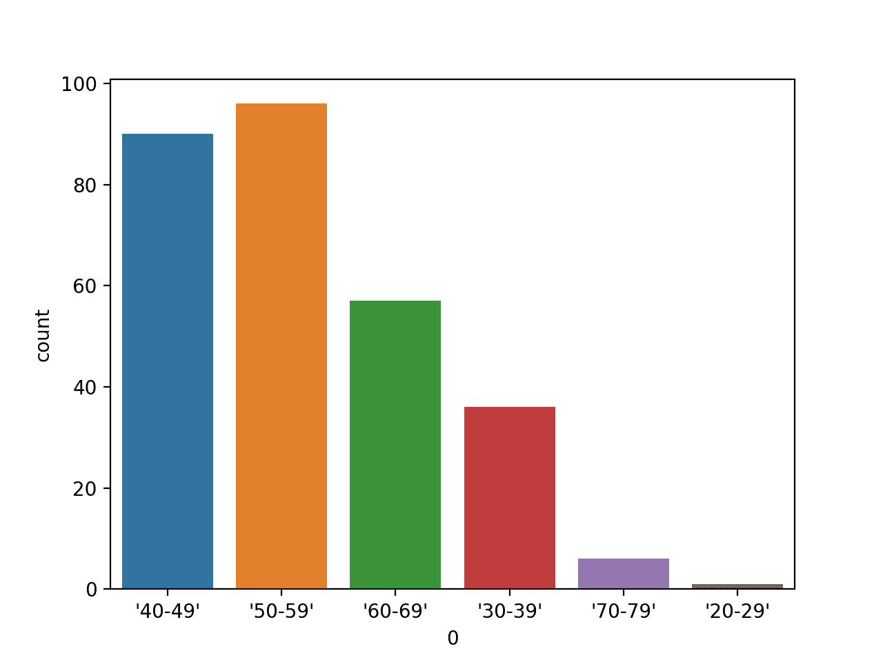
Bar Chart Plot of Age Range Categorical Variable
We might also want to plot the counts for each category for a variable, such as the first variable, against the class label.
This can be achieved using the countplot() function and specifying the class variable (column index 9) via the “hue” argument, as follows:
...
# create bar chart plot
countplot(x=0, hue=9, data=dataset)
Tying this together, the complete example is listed below.
# bar chart plot of a categorical variable against a class variable
from pandas import read_csv
from seaborn import countplot
from matplotlib import pyplot
# load the dataset
url = 'https://raw.githubusercontent.com/jbrownlee/Datasets/master/breast-cancer.csv'
dataset = read_csv(url, header=None)
# create bar chart plot
countplot(x=0, hue=9, data=dataset)
# show plot
pyplot.show()
Running the example first loads the breast cancer dataset and creates a bar chart plot of the data, showing each age group and the number of individuals (samples) that fall within each group separated by the two class labels for the dataset.
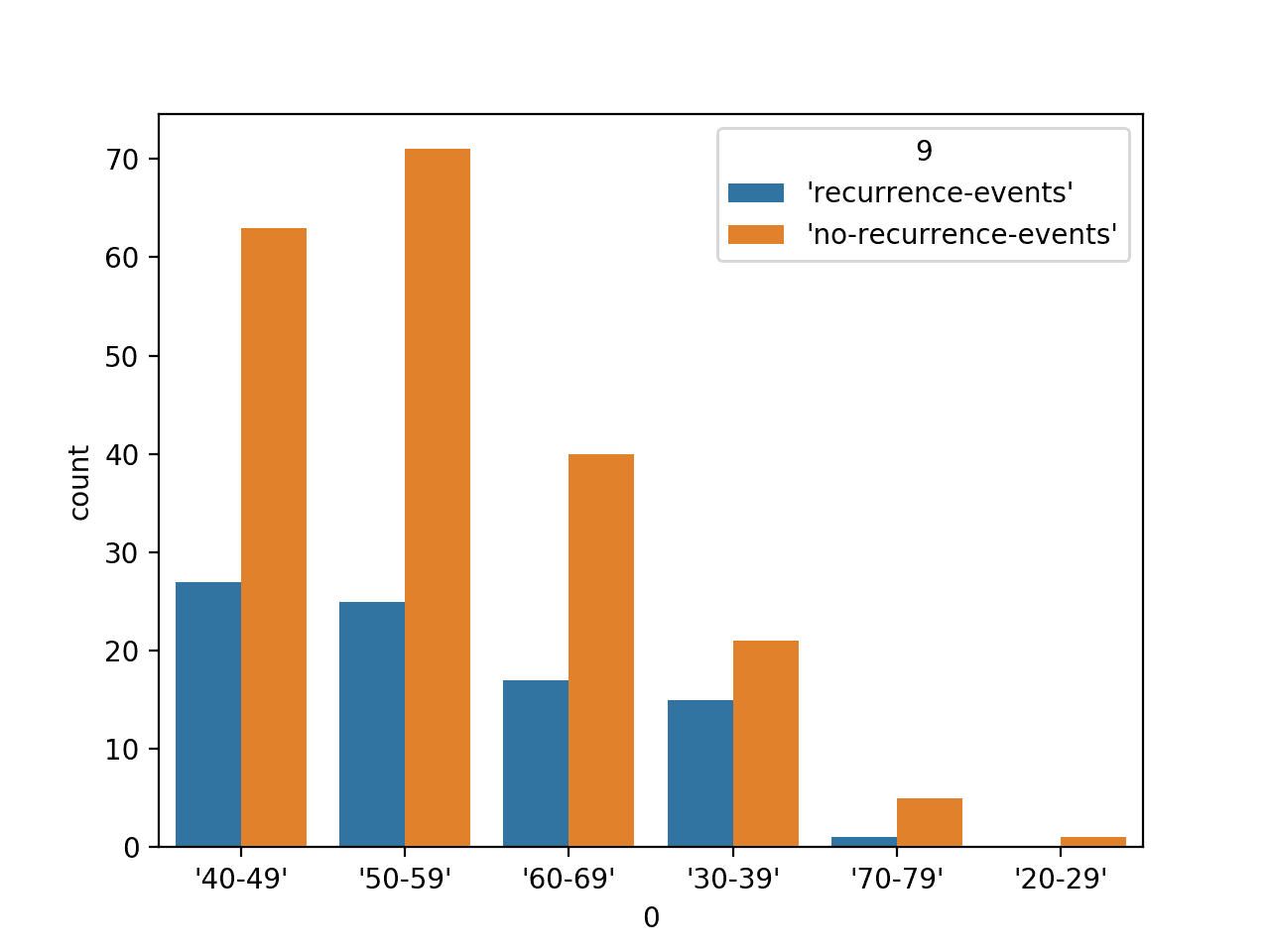
Bar Chart Plot of Age Range Categorical Variable by Class Label
For more great examples of bar chart plots with Seaborn, see: Plotting with categorical data.
Histogram Plots
A histogram plot is generally used to summarize the distribution of a numerical data sample.
The x-axis represents discrete bins or intervals for the observations. For example, observations with values between 1 and 10 may be split into five bins, the values [1,2] would be allocated to the first bin, [3,4] would be allocated to the second bin, and so on.
The y-axis represents the frequency or count of the number of observations in the dataset that belong to each bin.
Essentially, a data sample is transformed into a bar chart where each category on the x-axis represents an interval of observation values.
A histogram can be created in Seaborn by calling the distplot() function and passing the variable.
We will demonstrate a boxplot with a numerical variable from the diabetes classification dataset. We will just plot one variable, in this case, the first variable, which is the number of times that a patient was pregnant.
...
# create histogram plot
distplot(dataset[[0]])
Tying this together, the complete example is listed below.
# histogram plot of a numerical variable
from pandas import read_csv
from seaborn import distplot
from matplotlib import pyplot
# load the dataset
url = 'https://raw.githubusercontent.com/jbrownlee/Datasets/master/pima-indians-diabetes.csv'
dataset = read_csv(url, header=None)
# create histogram plot
distplot(dataset[[0]])
# show plot
pyplot.show()
Running the example first loads the diabetes dataset and creates a histogram plot of the variable, showing the distribution of the values with a hard cut-off at zero.
The plot shows both the histogram (counts of bins) as well as a smooth estimate of the probability density function.
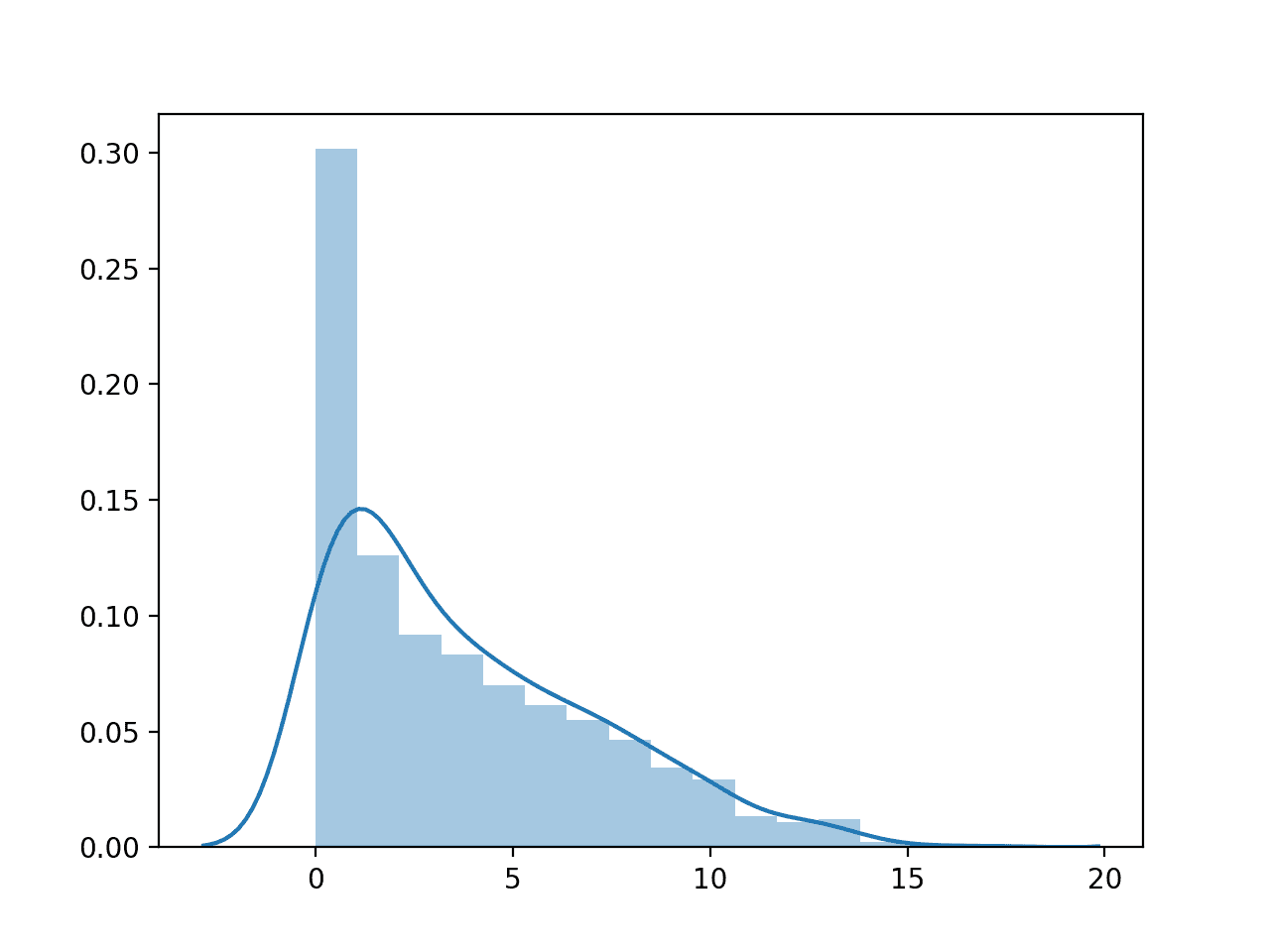
Histogram Plot of Number of Times Pregnant Numerical Variable
For more great examples of histogram plots with Seaborn, see: Visualizing the distribution of a dataset.
Box and Whisker Plots
A box and whisker plot, or boxplot for short, is generally used to summarize the distribution of a data sample.
The x-axis is used to represent the data sample, where multiple boxplots can be drawn side by side on the x-axis if desired.
The y-axis represents the observation values. A box is drawn to summarize the middle 50 percent of the dataset starting at the observation at the 25th percentile and ending at the 75th percentile. This is called the interquartile range, or IQR. The median, or 50th percentile, is drawn with a line.
Lines called whiskers are drawn extending from both ends of the box, calculated as (1.5 * IQR) to demonstrate the expected range of sensible values in the distribution. Observations outside the whiskers might be outliers and are drawn with small circles.
A boxplot can be created in Seaborn by calling the boxplot() function and passing the data.
We will demonstrate a boxplot with a numerical variable from the diabetes classification dataset. We will just plot one variable, in this case, the first variable, which is the number of times that a patient was pregnant.
...
# create box and whisker plot
boxplot(x=0, data=dataset)
Tying this together, the complete example is listed below.
# box and whisker plot of a numerical variable
from pandas import read_csv
from seaborn import boxplot
from matplotlib import pyplot
# load the dataset
url = 'https://raw.githubusercontent.com/jbrownlee/Datasets/master/pima-indians-diabetes.csv'
dataset = read_csv(url, header=None)
# create box and whisker plot
boxplot(x=0, data=dataset)
# show plot
pyplot.show()
Running the example first loads the diabetes dataset and creates a boxplot plot of the first input variable, showing the distribution of the number of times patients were pregnant.
We can see the median just above 2.5 times, some outliers up around 15 times (wow!).
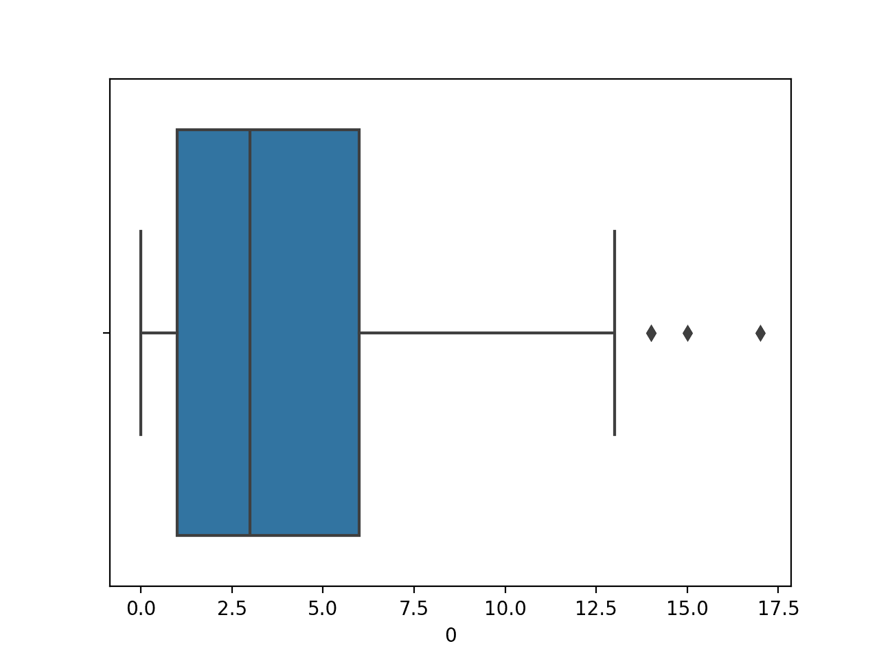
Box and Whisker Plot of Number of Times Pregnant Numerical Variable
We might also want to plot the distribution of the numerical variable for each value of a categorical variable, such as the first variable, against the class label.
This can be achieved by calling the boxplot() function and passing the class variable as the x-axis and the numerical variable as the y-axis.
...
# create box and whisker plot
boxplot(x=8, y=0, data=dataset)
Tying this together, the complete example is listed below.
# box and whisker plot of a numerical variable vs class label
from pandas import read_csv
from seaborn import boxplot
from matplotlib import pyplot
# load the dataset
url = 'https://raw.githubusercontent.com/jbrownlee/Datasets/master/pima-indians-diabetes.csv'
dataset = read_csv(url, header=None)
# create box and whisker plot
boxplot(x=8, y=0, data=dataset)
# show plot
pyplot.show()
Running the example first loads the diabetes dataset and creates a boxplot of the data, showing the distribution of the number of times pregnant as a numerical variable for the two-class labels.
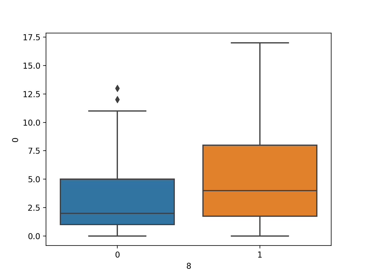
Box and Whisker Plot of Number of Times Pregnant Numerical Variable by Class Label
Scatter Plots
A scatter plot, or scatterplot, is generally used to summarize the relationship between two paired data samples.
Paired data samples mean that two measures were recorded for a given observation, such as the weight and height of a person.
The x-axis represents observation values for the first sample, and the y-axis represents the observation values for the second sample. Each point on the plot represents a single observation.
A scatterplot can be created in Seaborn by calling the scatterplot() function and passing the two numerical variables.
We will demonstrate a scatterplot with two numerical variables from the diabetes classification dataset. We will plot the first versus the second variable, in this case, the first variable, which is the number of times that a patient was pregnant, and the second is the plasma glucose concentration after a two hour oral glucose tolerance test (more details of the variables here).
...
# create scatter plot
scatterplot(x=0, y=1, data=dataset)
Tying this together, the complete example is listed below.
# scatter plot of two numerical variables
from pandas import read_csv
from seaborn import scatterplot
from matplotlib import pyplot
# load the dataset
url = 'https://raw.githubusercontent.com/jbrownlee/Datasets/master/pima-indians-diabetes.csv'
dataset = read_csv(url, header=None)
# create scatter plot
scatterplot(x=0, y=1, data=dataset)
# show plot
pyplot.show()
Running the example first loads the diabetes dataset and creates a scatter plot of the first two input variables.
We can see a somewhat uniform relationship between the two variables.
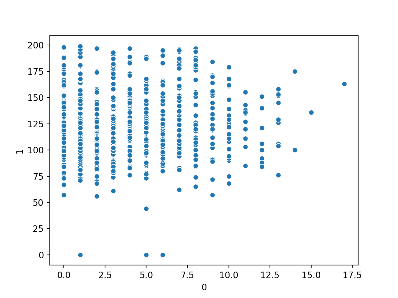
Scatter Plot of Number of Times Pregnant vs. Plasma Glucose Numerical Variables
We might also want to plot the relationship for the pair of numerical variables against the class label.
This can be achieved using the scatterplot() function and specifying the class variable (column index 8) via the “hue” argument, as follows:
...
# create scatter plot
scatterplot(x=0, y=1, hue=8, data=dataset)
Tying this together, the complete example is listed below.
# scatter plot of two numerical variables vs class label
from pandas import read_csv
from seaborn import scatterplot
from matplotlib import pyplot
# load the dataset
url = 'https://raw.githubusercontent.com/jbrownlee/Datasets/master/pima-indians-diabetes.csv'
dataset = read_csv(url, header=None)
# create scatter plot
scatterplot(x=0, y=1, hue=8, data=dataset)
# show plot
pyplot.show()
Running the example first loads the diabetes dataset and creates a scatter plot of the first two variables vs. class label.
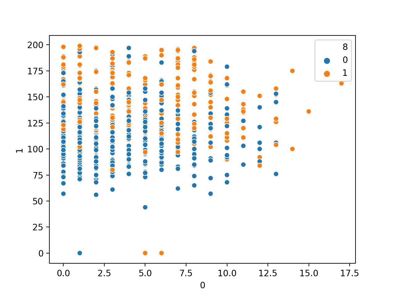
Scatter Plot of Number of Times Pregnant vs. Plasma Glucose Numerical Variables by Class Label
Further Reading
This section provides more resources on the topic if you are looking to go deeper.
Tutorials
APIs
Summary
In this tutorial, you discovered a gentle introduction to Seaborn data visualization for machine learning.
Specifically, you learned:
- How to summarize the distribution of variables using bar charts, histograms, and box and whisker plots.
- How to summarize relationships using line plots and scatter plots.
- How to compare the distribution and relationships of variables for different class values on the same plot.
Do you have any questions?
Ask your questions in the comments below and I will do my best to answer.
The post How to use Seaborn Data Visualization for Machine Learning appeared first on Machine Learning Mastery.
Ai
via https://www.AiUpNow.com
August 9, 2020 at 03:00PM by Jason Brownlee, Khareem Sudlow
