Clustering or cluster analysis is an unsupervised learning problem.
It is often used as a data analysis technique for discovering interesting patterns in data, such as groups of customers based on their behavior.
There are many clustering algorithms to choose from and no single best clustering algorithm for all cases. Instead, it is a good idea to explore a range of clustering algorithms and different configurations for each algorithm.
In this tutorial, you will discover how to fit and use top clustering algorithms in python.
After completing this tutorial, you will know:
- Clustering is an unsupervised problem of finding natural groups in the feature space of input data.
- There are many different clustering algorithms and no single best method for all datasets.
- How to implement, fit, and use top clustering algorithms in Python with the scikit-learn machine learning library.
Let’s get started.

Clustering Algorithms With Python
Photo by Lars Plougmann, some rights reserved.
Tutorial Overview
This tutorial is divided into three parts; they are:
- Clustering
- Clustering Algorithms
- Examples of Clustering Algorithms
- Library Installation
- Clustering Dataset
- Affinity Propagation
- Agglomerative Clustering
- BIRCH
- DBSCAN
- K-Means
- Mini-Batch K-Means
- Mean Shift
- OPTICS
- Spectral Clustering
- Gaussian Mixture Model
Clustering
Cluster analysis, or clustering, is an unsupervised machine learning task.
It involves automatically discovering natural grouping in data. Unlike supervised learning (like predictive modeling), clustering algorithms only interpret the input data and find natural groups or clusters in feature space.
Clustering techniques apply when there is no class to be predicted but rather when the instances are to be divided into natural groups.
— Page 141, Data Mining: Practical Machine Learning Tools and Techniques, 2016.
A cluster is often an area of density in the feature space where examples from the domain (observations or rows of data) are closer to the cluster than other clusters. The cluster may have a center (the centroid) that is a sample or a point feature space and may have a boundary or extent.
These clusters presumably reflect some mechanism at work in the domain from which instances are drawn, a mechanism that causes some instances to bear a stronger resemblance to each other than they do to the remaining instances.
— Pages 141-142, Data Mining: Practical Machine Learning Tools and Techniques, 2016.
Clustering can be helpful as a data analysis activity in order to learn more about the problem domain, so-called pattern discovery or knowledge discovery.
For example:
- The phylogenetic tree could be considered the result of a manual clustering analysis.
- Separating normal data from outliers or anomalies may be considered a clustering problem.
- Separating clusters based on their natural behavior is a clustering problem, referred to as market segmentation.
Clustering can also be useful as a type of feature engineering, where existing and new examples can be mapped and labeled as belonging to one of the identified clusters in the data.
Evaluation of identified clusters is subjective and may require a domain expert, although many clustering-specific quantitative measures do exist. Typically, clustering algorithms are compared academically on synthetic datasets with pre-defined clusters, which an algorithm is expected to discover.
Clustering is an unsupervised learning technique, so it is hard to evaluate the quality of the output of any given method.
— Page 534, Machine Learning: A Probabilistic Perspective, 2012.
Clustering Algorithms
There are many types of clustering algorithms.
Many algorithms use similarity or distance measures between examples in the feature space in an effort to discover dense regions of observations. As such, it is often good practice to scale data prior to using clustering algorithms.
Central to all of the goals of cluster analysis is the notion of the degree of similarity (or dissimilarity) between the individual objects being clustered. A clustering method attempts to group the objects based on the definition of similarity supplied to it.
— Page 502, The Elements of Statistical Learning: Data Mining, Inference, and Prediction, 2016.
Some clustering algorithms require you to specify or guess at the number of clusters to discover in the data, whereas others require the specification of some minimum distance between observations in which examples may be considered “close” or “connected.”
As such, cluster analysis is an iterative process where subjective evaluation of the identified clusters is fed back into changes to algorithm configuration until a desired or appropriate result is achieved.
The scikit-learn library provides a suite of different clustering algorithms to choose from.
A list of 10 of the more popular algorithms is as follows:
- Affinity Propagation
- Agglomerative Clustering
- BIRCH
- DBSCAN
- K-Means
- Mini-Batch K-Means
- Mean Shift
- OPTICS
- Spectral Clustering
- Mixture of Gaussians
Each algorithm offers a different approach to the challenge of discovering natural groups in data.
There is no best clustering algorithm, and no easy way to find the best algorithm for your data without using controlled experiments.
In this tutorial, we will review how to use each of these 10 popular clustering algorithms from the scikit-learn library.
The examples will provide the basis for you to copy-paste the examples and test the methods on your own data.
We will not dive into the theory behind how the algorithms work or compare them directly. For a good starting point on this topic, see:
Let’s dive in.
Examples of Clustering Algorithms
In this section, we will review how to use 10 popular clustering algorithms in scikit-learn.
This includes an example of fitting the model and an example of visualizing the result.
The examples are designed for you to copy-paste into your own project and apply the methods to your own data.
Library Installation
First, let’s install the library.
Don’t skip this step as you will need to ensure you have the latest version installed.
You can install the scikit-learn library using the pip Python installer, as follows:
sudo pip install scikit-learn
For additional installation instructions specific to your platform, see:
Next, let’s confirm that the library is installed and you are using a modern version.
Run the following script to print the library version number.
# check scikit-learn version
import sklearn
print(sklearn.__version__)
Running the example, you should see the following version number or higher.
0.22.1
Clustering Dataset
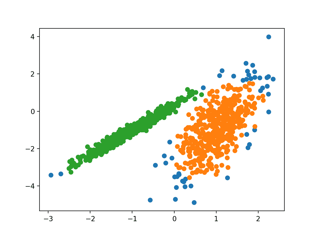
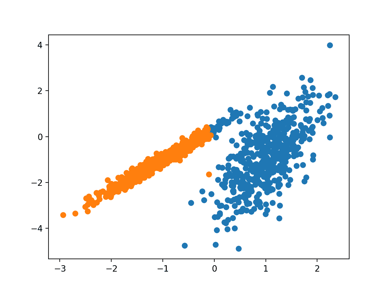
We will use the make_classification() function to create a test binary classification dataset.
The dataset will have 1,000 examples, with two input features and one cluster per class. The clusters are visually obvious in two dimensions so that we can plot the data with a scatter plot and color the points in the plot by the assigned cluster. This will help to see, at least on the test problem, how “well” the clusters were identified.
The clusters in this test problem are based on a multivariate Gaussian, and not all clustering algorithms will be effective at identifying these types of clusters. As such, the results in this tutorial should not be used as the basis for comparing the methods generally.
An example of creating and summarizing the synthetic clustering dataset is listed below.
# synthetic classification dataset
from numpy import where
from sklearn.datasets import make_classification
from matplotlib import pyplot
# define dataset
X, y = make_classification(n_samples=1000, n_features=2, n_informative=2, n_redundant=0, n_clusters_per_class=1, random_state=4)
# create scatter plot for samples from each class
for class_value in range(2):
        # get row indexes for samples with this class
        row_ix = where(y == class_value)
        # create scatter of these samples
        pyplot.scatter(X[row_ix, 0], X[row_ix, 1])
# show the plot
pyplot.show()
Running the example creates the synthetic clustering dataset, then creates a scatter plot of the input data with points colored by class label (idealized clusters).
We can clearly see two distinct groups of data in two dimensions and the hope would be that an automatic clustering algorithm can detect these groupings.
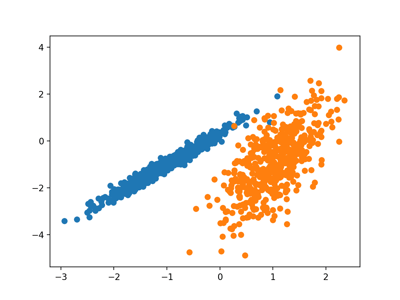
Scatter Plot of Synthetic Clustering Dataset With Points Colored by Known Cluster
Next, we can start looking at examples of clustering algorithms applied to this dataset.
I have made some minimal attempts to tune each method to the dataset.
Can you get a better result for one of the algorithms?
Let me know in the comments below.
Affinity Propagation
Affinity Propagation involves finding a set of exemplars that best summarize the data.
We devised a method called “affinity propagation,” which takes as input measures of similarity between pairs of data points. Real-valued messages are exchanged between data points until a high-quality set of exemplars and corresponding clusters gradually emerges
— Clustering by Passing Messages Between Data Points, 2007.
The technique is described in the paper:
It is implemented via the AffinityPropagation class and the main configuration to tune is the “damping” set between 0.5 and 1, and perhaps “preference.”
The complete example is listed below.
# affinity propagation clustering
from numpy import unique
from numpy import where
from sklearn.datasets import make_classification
from sklearn.cluster import AffinityPropagation
from matplotlib import pyplot
# define dataset
X, _ = make_classification(n_samples=1000, n_features=2, n_informative=2, n_redundant=0, n_clusters_per_class=1, random_state=4)
# define the model
model = AffinityPropagation(damping=0.9)
# fit the model
model.fit(X)
# assign a cluster to each example
yhat = model.predict(X)
# retrieve unique clusters
clusters = unique(yhat)
# create scatter plot for samples from each cluster
for cluster in clusters:
        # get row indexes for samples with this cluster
        row_ix = where(yhat == cluster)
        # create scatter of these samples
        pyplot.scatter(X[row_ix, 0], X[row_ix, 1])
# show the plot
pyplot.show()
Running the example fits the model on the training dataset and predicts a cluster for each example in the dataset. A scatter plot is then created with points colored by their assigned cluster.
In this case, I could not achieve a good result.
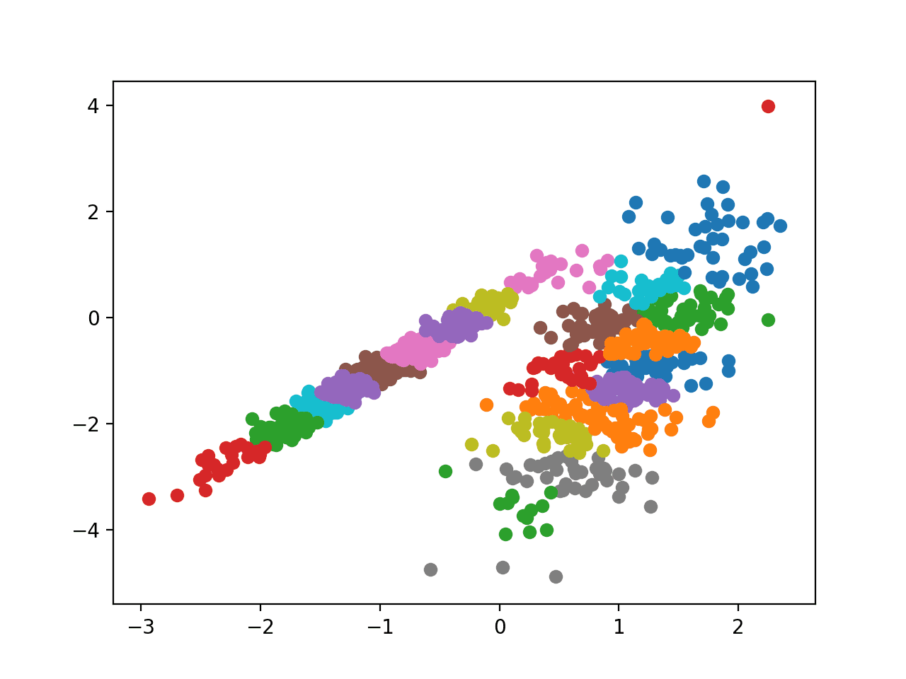
Scatter Plot of Dataset With Clusters Identified Using Affinity Propagation
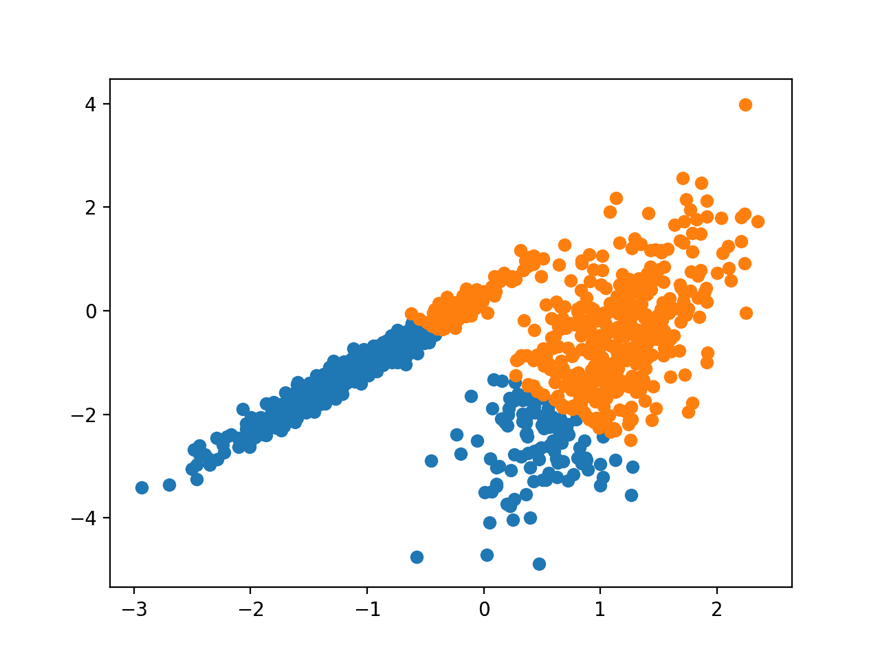
Agglomerative Clustering
Agglomerative clustering involves merging examples until the desired number of clusters is achieved.
It is a part of a broader class of hierarchical clustering methods and you can learn more here:
It is implemented via the AgglomerativeClustering class and the main configuration to tune is the “n_clusters” set, an estimate of the number of clusters in the data, e.g. 2.
The complete example is listed below.
# agglomerative clustering
from numpy import unique
from numpy import where
from sklearn.datasets import make_classification
from sklearn.cluster import AgglomerativeClustering
from matplotlib import pyplot
# define dataset
X, _ = make_classification(n_samples=1000, n_features=2, n_informative=2, n_redundant=0, n_clusters_per_class=1, random_state=4)
# define the model
model = AgglomerativeClustering(n_clusters=2)
# fit model and predict clusters
yhat = model.fit_predict(X)
# retrieve unique clusters
clusters = unique(yhat)
# create scatter plot for samples from each cluster
for cluster in clusters:
        # get row indexes for samples with this cluster
        row_ix = where(yhat == cluster)
        # create scatter of these samples
        pyplot.scatter(X[row_ix, 0], X[row_ix, 1])
# show the plot
pyplot.show()
Running the example fits the model on the training dataset and predicts a cluster for each example in the dataset. A scatter plot is then created with points colored by their assigned cluster.
In this case, a reasonable grouping is found.
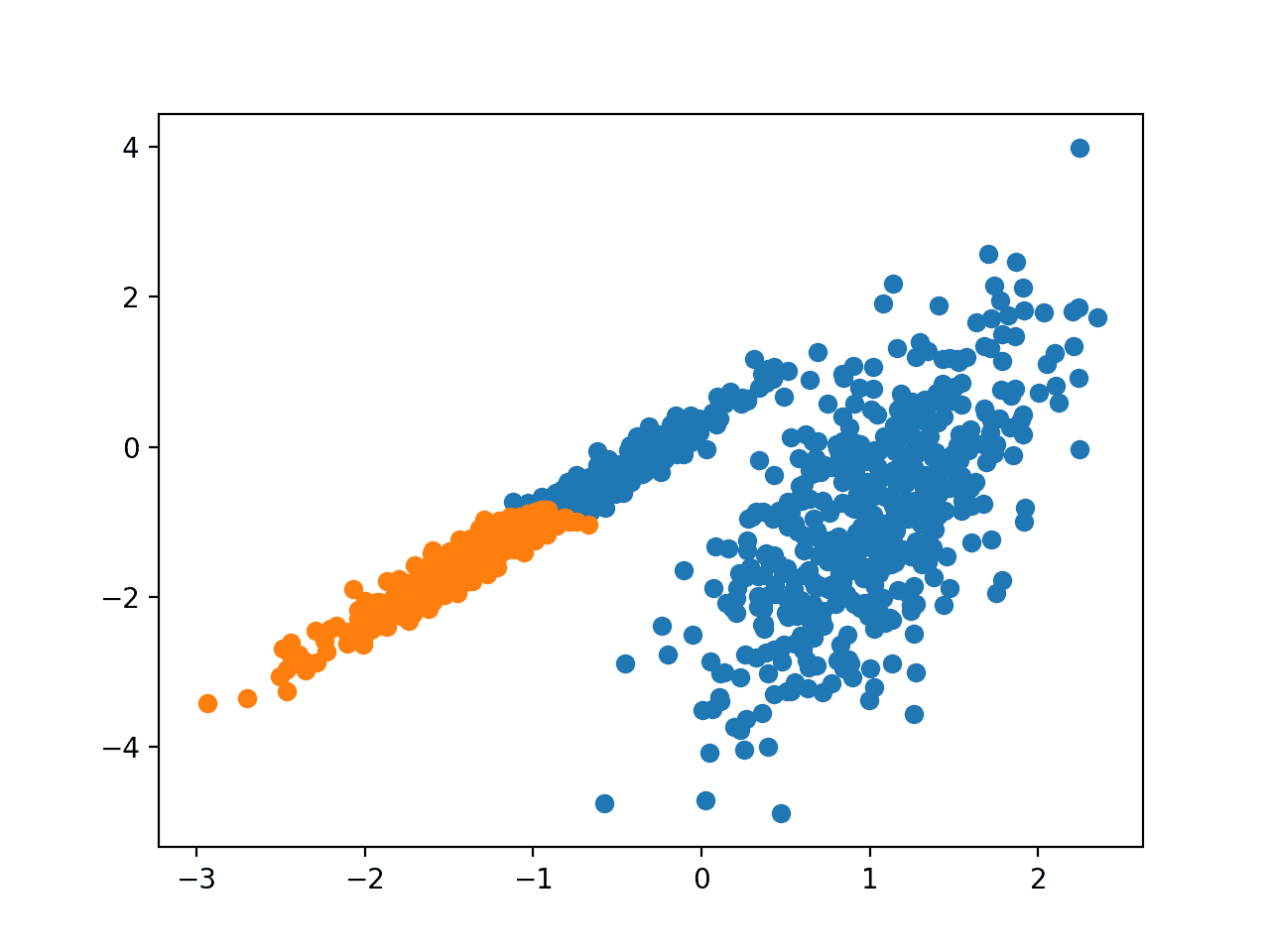
Scatter Plot of Dataset With Clusters Identified Using Agglomerative Clustering
BIRCH
BIRCH Clustering (BIRCH is short for Balanced Iterative Reducing and Clustering using
Hierarchies) involves constructing a tree structure from which cluster centroids are extracted.
BIRCH incrementally and dynamically clusters incoming multi-dimensional metric data points to try to produce the best quality clustering with the available resources (i. e., available memory and time constraints).
— BIRCH: An efficient data clustering method for large databases, 1996.
The technique is described in the paper:
It is implemented via the Birch class and the main configuration to tune is the “threshold” and “n_clusters” hyperparameters, the latter of which provides an estimate of the number of clusters.
The complete example is listed below.
# birch clustering
from numpy import unique
from numpy import where
from sklearn.datasets import make_classification
from sklearn.cluster import Birch
from matplotlib import pyplot
# define dataset
X, _ = make_classification(n_samples=1000, n_features=2, n_informative=2, n_redundant=0, n_clusters_per_class=1, random_state=4)
# define the model
model = Birch(threshold=0.01, n_clusters=2)
# fit the model
model.fit(X)
# assign a cluster to each example
yhat = model.predict(X)
# retrieve unique clusters
clusters = unique(yhat)
# create scatter plot for samples from each cluster
for cluster in clusters:
        # get row indexes for samples with this cluster
        row_ix = where(yhat == cluster)
        # create scatter of these samples
        pyplot.scatter(X[row_ix, 0], X[row_ix, 1])
# show the plot
pyplot.show()
Running the example fits the model on the training dataset and predicts a cluster for each example in the dataset. A scatter plot is then created with points colored by their assigned cluster.
In this case, an excellent grouping is found.
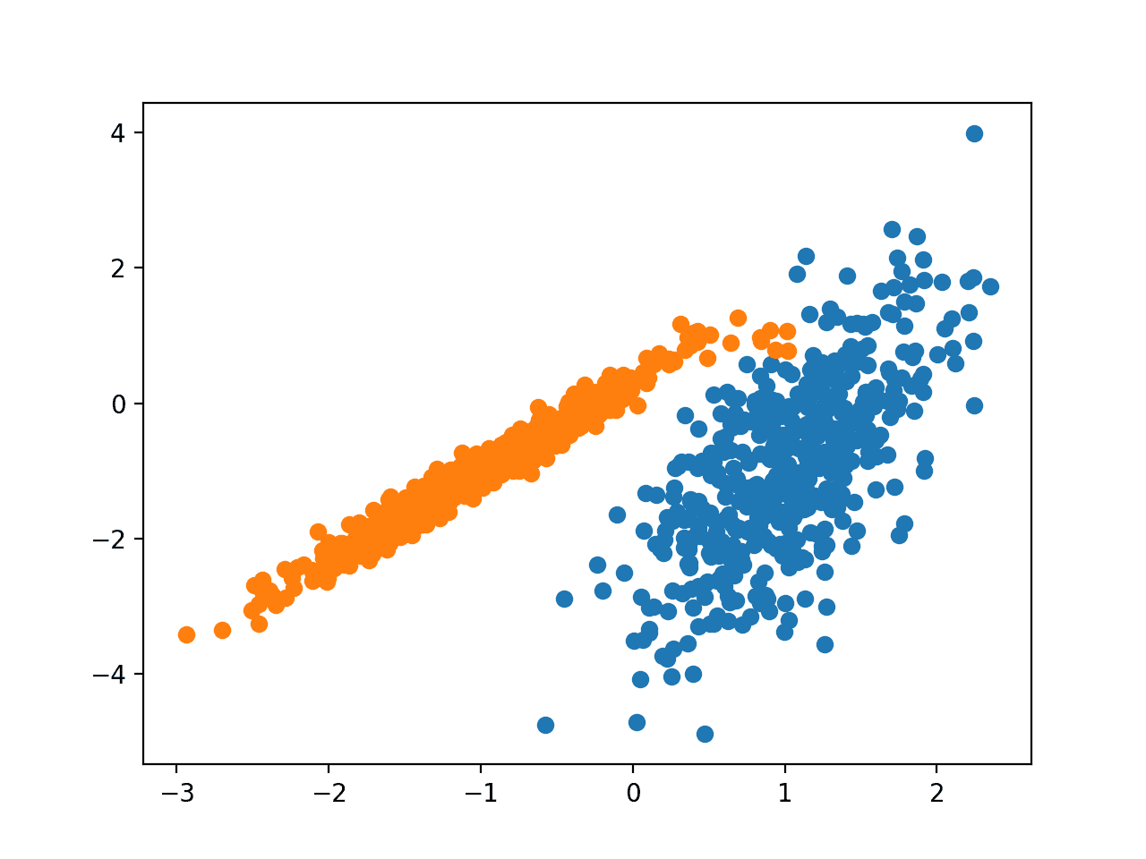
Scatter Plot of Dataset With Clusters Identified Using BIRCH Clustering
DBSCAN
DBSCAN Clustering (where DBSCAN is short for Density-Based Spatial Clustering of Applications with Noise) involves finding high-density areas in the domain and expanding those areas of the feature space around them as clusters.
… we present the new clustering algorithm DBSCAN relying on a density-based notion of clusters which is designed to discover clusters of arbitrary shape. DBSCAN requires only one input parameter and supports the user in determining an appropriate value for it
— A Density-Based Algorithm for Discovering Clusters in Large Spatial Databases with Noise, 1996.
The technique is described in the paper:
It is implemented via the DBSCAN class and the main configuration to tune is the “eps” and “min_samples” hyperparameters.
The complete example is listed below.
# dbscan clustering
from numpy import unique
from numpy import where
from sklearn.datasets import make_classification
from sklearn.cluster import DBSCAN
from matplotlib import pyplot
# define dataset
X, _ = make_classification(n_samples=1000, n_features=2, n_informative=2, n_redundant=0, n_clusters_per_class=1, random_state=4)
# define the model
model = DBSCAN(eps=0.30, min_samples=9)
# fit model and predict clusters
yhat = model.fit_predict(X)
# retrieve unique clusters
clusters = unique(yhat)
# create scatter plot for samples from each cluster
for cluster in clusters:
        # get row indexes for samples with this cluster
        row_ix = where(yhat == cluster)
        # create scatter of these samples
        pyplot.scatter(X[row_ix, 0], X[row_ix, 1])
# show the plot
pyplot.show()
Running the example fits the model on the training dataset and predicts a cluster for each example in the dataset. A scatter plot is then created with points colored by their assigned cluster.
In this case, a reasonable grouping is found, although more tuning is required.
Scatter Plot of Dataset With Clusters Identified Using DBSCAN Clustering
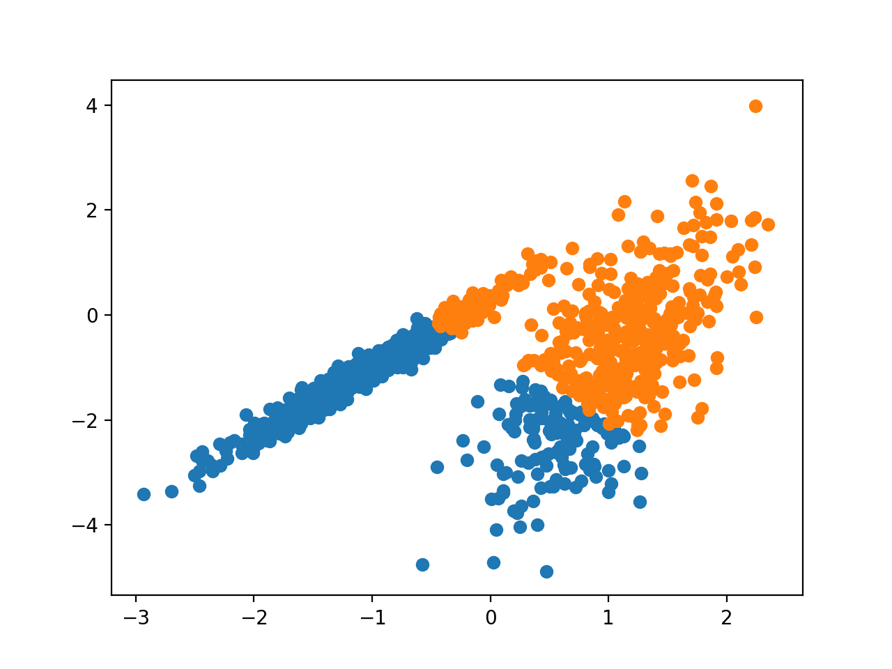
K-Means
K-Means Clustering may be the most widely known clustering algorithm and involves assigning examples to clusters in an effort to minimize the variance within each cluster.
The main purpose of this paper is to describe a process for partitioning an N-dimensional population into k sets on the basis of a sample. The process, which is called ‘k-means,’ appears to give partitions which are reasonably efficient in the sense of within-class variance.
— Some methods for classification and analysis of multivariate observations, 1967.
The technique is described here:
It is implemented via the KMeans class and the main configuration to tune is the “n_clusters” hyperparameter set to the estimated number of clusters in the data.
The complete example is listed below.
# k-means clustering
from numpy import unique
from numpy import where
from sklearn.datasets import make_classification
from sklearn.cluster import KMeans
from matplotlib import pyplot
# define dataset
X, _ = make_classification(n_samples=1000, n_features=2, n_informative=2, n_redundant=0, n_clusters_per_class=1, random_state=4)
# define the model
model = KMeans(n_clusters=2)
# fit the model
model.fit(X)
# assign a cluster to each example
yhat = model.predict(X)
# retrieve unique clusters
clusters = unique(yhat)
# create scatter plot for samples from each cluster
for cluster in clusters:
        # get row indexes for samples with this cluster
        row_ix = where(yhat == cluster)
        # create scatter of these samples
        pyplot.scatter(X[row_ix, 0], X[row_ix, 1])
# show the plot
pyplot.show()
Running the example fits the model on the training dataset and predicts a cluster for each example in the dataset. A scatter plot is then created with points colored by their assigned cluster.
In this case, a reasonable grouping is found, although the unequal equal variance in each dimension makes the method less suited to this dataset.
Scatter Plot of Dataset With Clusters Identified Using K-Means Clustering
Mini-Batch K-Means
Mini-Batch K-Means is a modified version of k-means that makes updates to the cluster centroids using mini-batches of samples rather than the entire dataset, which can make it faster for large datasets, and perhaps more robust to statistical noise.
… we propose the use of mini-batch optimization for k-means clustering. This reduces computation cost by orders of magnitude compared to the classic batch algorithm while yielding significantly better solutions than online stochastic gradient descent.
— Web-Scale K-Means Clustering, 2010.
The technique is described in the paper:
- Web-Scale K-Means Clustering, 2010.
It is implemented via the MiniBatchKMeans class and the main configuration to tune is the “n_clusters” hyperparameter set to the estimated number of clusters in the data.
The complete example is listed below.
# mini-batch k-means clustering
from numpy import unique
from numpy import where
from sklearn.datasets import make_classification
from sklearn.cluster import MiniBatchKMeans
from matplotlib import pyplot
# define dataset
X, _ = make_classification(n_samples=1000, n_features=2, n_informative=2, n_redundant=0, n_clusters_per_class=1, random_state=4)
# define the model
model = MiniBatchKMeans(n_clusters=2)
# fit the model
model.fit(X)
# assign a cluster to each example
yhat = model.predict(X)
# retrieve unique clusters
clusters = unique(yhat)
# create scatter plot for samples from each cluster
for cluster in clusters:
        # get row indexes for samples with this cluster
        row_ix = where(yhat == cluster)
        # create scatter of these samples
        pyplot.scatter(X[row_ix, 0], X[row_ix, 1])
# show the plot
pyplot.show()
Running the example fits the model on the training dataset and predicts a cluster for each example in the dataset. A scatter plot is then created with points colored by their assigned cluster.
In this case, a result equivalent to the standard k-means algorithm is found.
Scatter Plot of Dataset With Clusters Identified Using Mini-Batch K-Means Clustering
Mean Shift
Mean shift clustering involves finding and adapting centroids based on the density of examples in the feature space.
We prove for discrete data the convergence of a recursive mean shift procedure to the nearest stationary point of the underlying density function and thus its utility in detecting the modes of the density.
— Mean Shift: A robust approach toward feature space analysis, 2002.
The technique is described in the paper:
It is implemented via the MeanShift class and the main configuration to tune is the “bandwidth” hyperparameter.
The complete example is listed below.
# mean shift clustering
from numpy import unique
from numpy import where
from sklearn.datasets import make_classification
from sklearn.cluster import MeanShift
from matplotlib import pyplot
# define dataset
X, _ = make_classification(n_samples=1000, n_features=2, n_informative=2, n_redundant=0, n_clusters_per_class=1, random_state=4)
# define the model
model = MeanShift()
# fit model and predict clusters
yhat = model.fit_predict(X)
# retrieve unique clusters
clusters = unique(yhat)
# create scatter plot for samples from each cluster
for cluster in clusters:
        # get row indexes for samples with this cluster
        row_ix = where(yhat == cluster)
        # create scatter of these samples
        pyplot.scatter(X[row_ix, 0], X[row_ix, 1])
# show the plot
pyplot.show()
Running the example fits the model on the training dataset and predicts a cluster for each example in the dataset. A scatter plot is then created with points colored by their assigned cluster.
In this case, a reasonable set of clusters are found in the data.

Scatter Plot of Dataset With Clusters Identified Using Mean Shift Clustering
OPTICS
OPTICS clustering (where OPTICS is short for Ordering Points To Identify the Clustering Structure) is a modified version of DBSCAN described above.
We introduce a new algorithm for the purpose of cluster analysis which does not produce a clustering of a data set explicitly; but instead creates an augmented ordering of the database representing its density-based clustering structure. This cluster-ordering contains information which is equivalent to the density-based clusterings corresponding to a broad range of parameter settings.
— OPTICS: ordering points to identify the clustering structure, 1999.
The technique is described in the paper:
It is implemented via the OPTICS class and the main configuration to tune is the “eps” and “min_samples” hyperparameters.
The complete example is listed below.
# optics clustering
from numpy import unique
from numpy import where
from sklearn.datasets import make_classification
from sklearn.cluster import OPTICS
from matplotlib import pyplot
# define dataset
X, _ = make_classification(n_samples=1000, n_features=2, n_informative=2, n_redundant=0, n_clusters_per_class=1, random_state=4)
# define the model
model = OPTICS(eps=0.8, min_samples=10)
# fit model and predict clusters
yhat = model.fit_predict(X)
# retrieve unique clusters
clusters = unique(yhat)
# create scatter plot for samples from each cluster
for cluster in clusters:
        # get row indexes for samples with this cluster
        row_ix = where(yhat == cluster)
        # create scatter of these samples
        pyplot.scatter(X[row_ix, 0], X[row_ix, 1])
# show the plot
pyplot.show()
Running the example fits the model on the training dataset and predicts a cluster for each example in the dataset. A scatter plot is then created with points colored by their assigned cluster.
In this case, I could not achieve a reasonable result on this dataset.
Scatter Plot of Dataset With Clusters Identified Using OPTICS Clustering
Spectral Clustering
Spectral Clustering is a general class of clustering methods, drawn from linear algebra.
A promising alternative that has recently emerged in a number of fields is to use spectral methods for clustering. Here, one uses the top eigenvectors of a matrix derived from the distance between points.
— On Spectral Clustering: Analysis and an algorithm, 2002.
The technique is described in the paper:
It is implemented via the SpectralClustering class and the main Spectral Clustering is a general class of clustering methods, drawn from linear algebra. to tune is the “n_clusters” hyperparameter used to specify the estimated number of clusters in the data.
The complete example is listed below.
# spectral clustering
from numpy import unique
from numpy import where
from sklearn.datasets import make_classification
from sklearn.cluster import SpectralClustering
from matplotlib import pyplot
# define dataset
X, _ = make_classification(n_samples=1000, n_features=2, n_informative=2, n_redundant=0, n_clusters_per_class=1, random_state=4)
# define the model
model = SpectralClustering(n_clusters=2)
# fit model and predict clusters
yhat = model.fit_predict(X)
# retrieve unique clusters
clusters = unique(yhat)
# create scatter plot for samples from each cluster
for cluster in clusters:
        # get row indexes for samples with this cluster
        row_ix = where(yhat == cluster)
        # create scatter of these samples
        pyplot.scatter(X[row_ix, 0], X[row_ix, 1])
# show the plot
pyplot.show()
Running the example fits the model on the training dataset and predicts a cluster for each example in the dataset. A scatter plot is then created with points colored by their assigned cluster.
In this case, reasonable clusters were found.
Scatter Plot of Dataset With Clusters Identified Using Spectra Clustering Clustering
Gaussian Mixture Model
A Gaussian mixture model summarizes a multivariate probability density function with a mixture of Gaussian probability distributions as its name suggests.
For more on the model, see:
It is implemented via the GaussianMixture class and the main configuration to tune is the “n_clusters” hyperparameter used to specify the estimated number of clusters in the data.
The complete example is listed below.
# gaussian mixture clustering
from numpy import unique
from numpy import where
from sklearn.datasets import make_classification
from sklearn.mixture import GaussianMixture
from matplotlib import pyplot
# define dataset
X, _ = make_classification(n_samples=1000, n_features=2, n_informative=2, n_redundant=0, n_clusters_per_class=1, random_state=4)
# define the model
model = GaussianMixture(n_components=2)
# fit the model
model.fit(X)
# assign a cluster to each example
yhat = model.predict(X)
# retrieve unique clusters
clusters = unique(yhat)
# create scatter plot for samples from each cluster
for cluster in clusters:
        # get row indexes for samples with this cluster
        row_ix = where(yhat == cluster)
        # create scatter of these samples
        pyplot.scatter(X[row_ix, 0], X[row_ix, 1])
# show the plot
pyplot.show()
Running the example fits the model on the training dataset and predicts a cluster for each example in the dataset. A scatter plot is then created with points colored by their assigned cluster.
In this case, we can see that the clusters were identified perfectly. This is not surprising given that the dataset was generated as a mixture of Gaussians.

Scatter Plot of Dataset With Clusters Identified Using Gaussian Mixture Clustering
Further Reading
This section provides more resources on the topic if you are looking to go deeper.
Papers
- Clustering by Passing Messages Between Data Points, 2007.
- BIRCH: An efficient data clustering method for large databases, 1996.
- A Density-Based Algorithm for Discovering Clusters in Large Spatial Databases with Noise, 1996.
- Some methods for classification and analysis of multivariate observations, 1967.
- Web-Scale K-Means Clustering, 2010.
- Mean Shift: A robust approach toward feature space analysis, 2002.
- On Spectral Clustering: Analysis and an algorithm, 2002.
Books
- Data Mining: Practical Machine Learning Tools and Techniques, 2016.
- The Elements of Statistical Learning: Data Mining, Inference, and Prediction, 2016.
- Machine Learning: A Probabilistic Perspective, 2012.
APIs
Articles
- Cluster analysis, Wikipedia.
- Hierarchical clustering, Wikipedia.
- k-means clustering, Wikipedia.
- Mixture model, Wikipedia.
Summary
In this tutorial, you discovered how to fit and use top clustering algorithms in python.
Specifically, you learned:
- Clustering is an unsupervised problem of finding natural groups in the feature space of input data.
- There are many different clustering algorithms, and no single best method for all datasets.
- How to implement, fit, and use top clustering algorithms in Python with the scikit-learn machine learning library.
Do you have any questions?
Ask your questions in the comments below and I will do my best to answer.
The post 10 Clustering Algorithms With Python appeared first on Machine Learning Mastery.
Ai
via https://www.AiUpNow.com
April 5, 2020 at 03:23PM by Jason Brownlee, Khareem Sudlow
