Last Updated on October 4, 2022
With the Transformer architecture revolutionizing the implementation of attention, and achieving very promising results in the natural language processing domain, it was only a matter of time before we could see its application in the computer vision domain too. This was eventually achieved with the implementation of the Vision Transformer (ViT).
In this tutorial, you will discover the architecture of the Vision Transformer model, and its application to the task of image classification.
After completing this tutorial, you will know:
- How the ViT works in the context of image classification.
- What the training process of the ViT entails.
- How the ViT compares to convolutional neural networks in terms of inductive bias.
- How the ViT fares against ResNets on different datasets.
- How the data is processed internally for the ViT to achieve its performance.
Let’s get started.

The Vision Transformer Model
Photo by Paul Skorupskas, some rights reserved.
Tutorial Overview
This tutorial is divided into six parts; they are:
- Introduction to the Vision Transformer (ViT)
- The ViT Architecture
- Training the ViT
- Inductive Bias in Comparison to Convolutional Neural Networks
- Comparative Performance of ViT Variants with ResNets
- Internal Representation of Data
Prerequisites
For this tutorial, we assume that you are already familiar with:
Introduction to the Vision Transformer (ViT)
We had seen how the emergence of the Transformer architecture of Vaswani et al. (2017) has revolutionized the use of attention, without relying on recurrence and convolutions as earlier attention models had previously done. In their work, Vaswani et al. had applied their model to the specific problem of natural language processing (NLP).
In computer vision, however, convolutional architectures remain dominant …
– An Image is Worth 16×16 Words: Transformers for Image Recognition at Scale, 2021.
Inspired by its success in NLP, Dosovitskiy et al. (2021) sought to apply the standard Transformer architecture to images, as we shall see shortly. Their target application at the time was image classification.
The ViT Architecture
Recall that the standard Transformer model received a one-dimensional sequence of word embeddings as input, since it was originally meant for NLP. In contrast, when applied to the task of image classification in computer vision, the input data to the Transformer model is provided in the form of two-dimensional images.
For the purpose of structuring the input image data in a manner that resembles how the input is structured in the NLP domain (in the sense of having a sequence of individual words), the input image, of height $H$, width $W$, and $C$ number of channels, is cut up into smaller two-dimensional patches. This results into $N = \tfrac{HW}{P^2}$ number of patches, where each patch has a resolution of ($P, P$) pixels.
Before feeding the data into the Transformer, the following operations are applied:
- Each image patch is flattened into a vector, $\mathbf{x}_p^n$, of length $P^2 \times C$, where $n = 1, \dots N$.
- A sequence of embedded image patches is generated by mapping the flattened patches to $D$ dimensions, with a trainable linear projection, $\mathbf{E}$.
- A learnable class embedding, $\mathbf{x}_{\text{class}}$, is prepended to the sequence of embedded image patches. The value of $\mathbf{x}_{\text{class}}$ represents the classification output, $\mathbf{y}$.
- The patch embeddings are finally augmented with one-dimensional positional embeddings, $\mathbf{E}_{\text{pos}}$, hence introducing positional information into the input, which is also learned during training.
The sequence of embedding vectors that results from the aforementioned operations is the following:
$$\mathbf{z}_0 = [ \mathbf{x}_{\text{class}}; \; \mathbf{x}_p^1 \mathbf{E}; \; \dots ; \; \mathbf{x}_p^N \mathbf{E}] + \mathbf{E}_{\text{pos}}$$
Dosovitskiy et al. make use of the encoder part of the Transformer architecture of Vaswani et al.
In order to perform classification, they feed $\mathbf{z}_0$ at the input of the Transformer encoder, which consists of a stack of $L$ identical layers. Then, they proceed to take the value of $\mathbf{x}_{\text{class}}$ at the $L^{\text{th}}$ layer of the encoder output, and feed it into a classification head.
The classification head is implemented by a MLP with one hidden layer at pre-training time and by a single linear layer at fine-tuning time.
– An Image is Worth 16×16 Words: Transformers for Image Recognition at Scale, 2021.
The multilayer perceptron (MLP) that forms the classification head implements Gaussian Error Linear Unit (GELU) non-linearity.
In summary, therefore, the ViT employs the encoder part of the original Transformer architecture. The input to the encoder is a sequence of embedded image patches (including a learnable class embedding prepended to the sequence), which is also augmented with positional information. A classification head attached to the output of the encoder receives the value of the learnable class embedding, to generate a classification output based on its state. All of this is illustrated by the figure below:
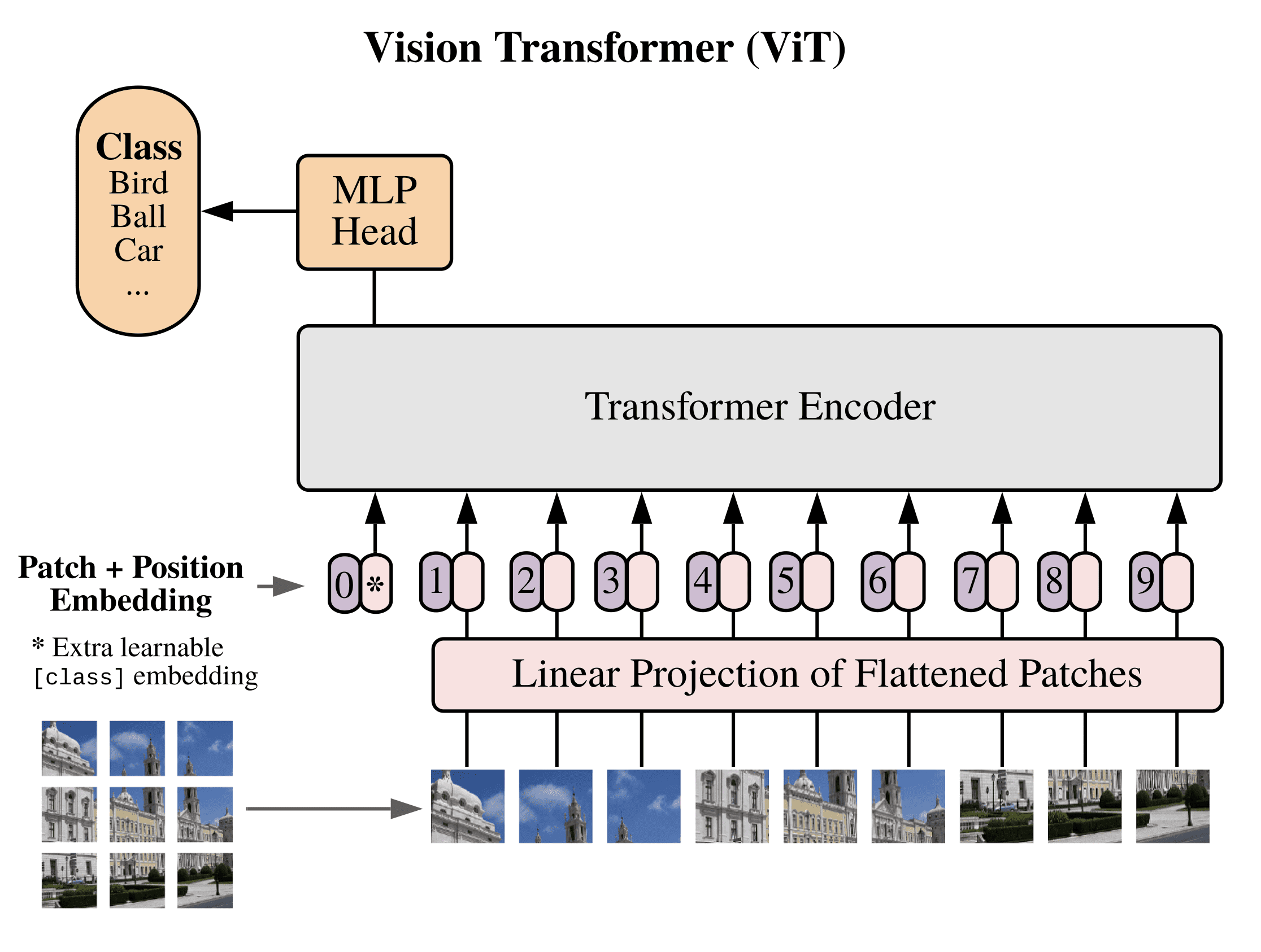
The Architecture of the Vision Transformer (ViT)
Taken from “An Image is Worth 16×16 Words: Transformers for Image Recognition at Scale“
One further note that Dosovitskiy et al. make, is that the original image can, alternatively, be fed into a convolutional neural network (CNN) before being passed on to the Transformer encoder. The sequence of image patches would then be obtained from the feature maps of the CNN, while the ensuing process of embedding the feature map patches, prepending a class token, and augmenting with positional information remains the same.
Training the ViT
The ViT is pre-trained on larger datasets (such as ImageNet, ImageNet-21k and JFT-300M) and fine-tuned to a smaller number of classes.
During pre-training, the classification head in use that is attached to the encoder output, is implemented by a MLP with one hidden layer and GELU non-linearity, as has been described earlier.
During fine-tuning, the MLP is replaced by a single (zero-initialized) feedforward layer of size, $D \times K$, with $K$ denoting the number of classes corresponding to the task at hand.
Fine-tuning is carried out on images that are of higher resolution than those used during pre-training, but the patch size into which the input images are cut is kept the same at all stages of training. This results in an input sequence of larger length at the fine-tuning stage, in comparison to that used during pre-training.
The implication of having a lengthier input sequence is that fine-tuning requires more position embeddings than pre-training. To circumvent this problem, Dosovitskiy et al. interpolate, in two-dimensions, the pre-training position embeddings according to their location in the original image, to obtain a longer sequence that matches the number of image patches in use during fine-tuning.
Inductive Bias in Comparison to Convolutional Neural Networks
Inductive bias refers to any assumptions that a model makes to generalise the training data and learn the target function.
In CNNs, locality, two-dimensional neighborhood structure, and translation equivariance are baked into each layer throughout the whole model.
– An Image is Worth 16×16 Words: Transformers for Image Recognition at Scale, 2021.
In convolutional neural networks (CNNs), each neuron is only connected to other neurons in its neighborhood. Furthermore, since neurons residing on the same layer share the same weight and bias values, any of these neurons will activate when a feature of interest falls within its receptive field. This results in a feature map that is equivariant to feature translation, which means that if the input image is translated, then the feature map is also equivalently translated.
Dosovitskiy et al. argue that in the ViT, only the MLP layers are characterised by locality and translation equivariance. The self-attention layers, on the other hand, are described as global, because the computations that are performed at these layers are not constrained to a local two-dimensional neighborhood.
They explain that bias about the two-dimensional neighborhood structure of the images is only used:
- At the input to the model, where each image is cut into patches, hence inherently retaining the spatial relationship between the pixels in each patch.
- At fine-tuning, where the pre-training position embeddings are interpolated in two-dimensions according to their location in the original image, to produce a longer sequence that matches the number of image patches in use during fine-tuning.
Comparative Performance of ViT Variants with ResNets
Dosovitskiy et al. pitted three ViT models of increasing size, against two modified ResNets of different sizes. Their experiments yield several interesting findings:
- Experiment 1 – Fine-tuning and testing on ImageNet:
- When pre-trained on the smallest dataset (ImageNet), the two larger ViT models underperformed in comparison to their smaller counterpart. The performance of all ViT models remains, generally, below that of the ResNets.
- When pre-trained on a larger dataset (ImageNet-21k), the three ViT models performed similarly to one another, as well as to the ResNets.
- When pre-trained on the largest dataset (JFT-300M), the performance of the larger ViT models overtakes the performance of the smaller ViT and the ResNets.
- Experiment 2 – Training on random subsets of different sizes of the JFT-300M dataset, and testing on ImageNet, to further investigate the effect of the dataset size:
- On smaller subsets of the dataset, the ViT models overfit more than the ResNet models, and underperform considerably.
- On the larger subset of the dataset, the performance of the larger ViT model surpasses the performance of the ResNets.
This result reinforces the intuition that the convolutional inductive bias is useful for smaller datasets, but for larger ones, learning the relevant patterns directly from data is sufficient, even beneficial.
– An Image is Worth 16×16 Words: Transformers for Image Recognition at Scale, 2021.
Internal Representation of Data
In analysing the internal representation of the image data in the ViT, Dosovitskiy et al. find the following:
- The learned embedding filters that are initially applied to the image patches at the first layer of the ViT, resemble basis functions that can extract the low-level features within each patch:

Learned Embedding Filters
Taken from “An Image is Worth 16×16 Words: Transformers for Image Recognition at Scale“
- Image patches that are spatially close to one another in the original image, are characterised by learned positional embeddings that are similar:
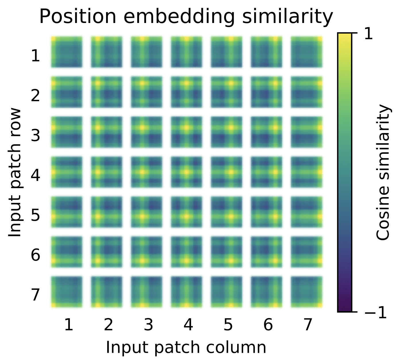
Learned Positional Embeddings
Taken from “An Image is Worth 16×16 Words: Transformers for Image Recognition at Scale“
- Several self-attention heads at the lowest layers of the model already attend to most of the image information (based on their attention weights), demonstrating the capability of the self-attention mechanism in integrating the information across the entire image:

Size of Image Area Attended by Different Self-Attention Heads
Taken from “An Image is Worth 16×16 Words: Transformers for Image Recognition at Scale“
Further Reading
This section provides more resources on the topic if you are looking to go deeper.
Papers
- An Image is Worth 16×16 Words: Transformers for Image Recognition at Scale, 2021.
- Attention Is All You Need, 2017.
Summary
In this tutorial, you discovered the architecture of the Vision Transformer model, and its application to the task of image classification.
Specifically, you learned:
- How the ViT works in the context of image classification.
- What the training process of the ViT entails.
- How the ViT compares to convolutional neural networks in terms of inductive bias.
- How the ViT fares against ResNets on different datasets.
- How the data is processed internally for the ViT to achieve its performance.
Do you have any questions?
Ask your questions in the comments below and I will do my best to answer.
The post The Vision Transformer Model appeared first on Machine Learning Mastery.
via https://AIupNow.com
Stefania Cristina, Khareem Sudlow
